Software & Projects
Research software and methodological packages developed as part of my work in Bayesian statistics and climate science.
- Replaces sliding windows with a model-based estimate of stability
- Jointly models the trend and the rising lag-one autocorrelation
- Separates correlated external variability with a nested AR(1) option
- Fast Bayesian inference using R-INLA
Critical slowing down refers to the generic dynamical phenomenon that occurs as a system approaches a bifurcation-induced tipping point, where the stability of an equilibrium state is progressively lost. As the dominant restoring forces weaken near the bifurcation, the system’s recovery from perturbations becomes increasingly slow, leading to a characteristic increase in the autocorrelation and variance of fluctuations. These statistical changes give rise to so-called early warning signals, which can be detected in time series data prior to a transition. In the context of bifurcation-induced tipping points, such signals provide indirect probabilistic evidence that a system is approaching a critical threshold, beyond which a small perturbation may trigger a qualitative shift to an alternative stable state.
Typically, early warning signals are estimated using a sliding windows approach. This can be problematic, especially for short time series, as it requires a choice for the window length. Short windows allow for better representation of the momentary state which can capture rapid changes in stability, but provides a more limited number of data points for estimation, leading to inaccurate estimates. Long windows improves precision, but may smooth out abrupt transitions making them harder to detect in time.
In Myrvoll-Nilsen et al. (2025) we suggest using a model-based approach where we approximate the time-dependent Ornstein-Uhlenbeck process using an AR(1) process where the lag-one autocorrelation parameter is expressed as a linear function of time. By implementing this into a latent Gaussian model framework we utilize the Markov property to enable efficient Bayesian inference using the R-INLA methodology (Rue et al., 2009). Early warning signals can then be detected from the posterior probability of the slope of the lag-one autocorrelation being positive.
Correlated external variability poses a challenge in early warning signal detection. Boers (2021) demonstrates that applying standard metrics to a stable system driven by correlated noise can lead to biased estimates and false positives. Morr and Boers (2024) suggests modeling the innovation as an AR(1) process. In Hallali et al. (2025) we extend on the framework by adopting a time-dependent version of this nested AR(1) model, allowing external variability to be modeled separately.
The time-dependent AR(1) model is included in the INLA.ews package using the model='ar1' option, while the nested time-dependent AR(1) model is available using the model='ar2' option.
- Boers, N. (2021). Observation-based early-warning signals for a collapse of the Atlantic Meridional Overturning Circulation. Nature Climate Change, 11(8), 680–688. doi:10.1038/s41558-021-01097-4
- Hallali, L., Myrvoll-Nilsen, E. and Franzke, C. L. (2025). Assessing AMOC stability using a Bayesian nested time-dependent autoregressive model. Nonlinear Processes in Geophysics, 32(4), 383–395. doi:10.5194/npg-32-383-2025
- Morr, A. and Boers, N. (2024). Detection of approaching critical transitions in natural systems driven by red noise. Physical Review X, 14, 021037. doi:10.1103/PhysRevX.14.021037
- Myrvoll-Nilsen, E., Hallali, L. and Rypdal, M. (2025). Bayesian analysis of early warning signals using a time-dependent model. Earth System Dynamics, 16(5), 1539–1556. doi:10.5194/esd-16-1539-2025
- Rue, H., Martino, S. and Chopin, N. (2009). Approximate Bayesian inference for latent Gaussian models by using integrated nested Laplace approximations. Journal of the Royal Statistical Society: Series B, 71(2), 319–392. doi:10.1111/j.1467-9868.2008.00700.x
- Make sure you have R installed (https://cran.r-project.org)
- Install INLA (https://www.r-inla.org/download/)
library(remotes)
remotes::install_github('eirikmn/INLA.ews')set.seed(1)
n = 500
time = 1:n
phis = seq(0.4,0.7,length.out=n)
data = ar1_timedep_sim(n,sigma=1,phis=phis)
object = inla.ews(data,model='ar1')
summary(object)
plot(object)Call:
inla.ews(data, model = 'ar1')
Time used:
Running INLA Post processing Total
3.8047 31.4884 35.5473
Posterior marginal distributions for all parameters have been computed.
Summary statistics for fixed effects:
mean sd 0.025quant 0.5quant 0.975quant
(Intercept) 0.0442 0.0715 -0.096 0.0441 0.1851
Summary statistics using ar1 model:
mean sd 0.025quant 0.5quant 0.975quant
a 0.3120 0.0548 0.2108 0.3095 0.4243
b 0.3535 0.0633 0.2255 0.3547 0.4736
sigma 1.0618 0.0684 0.9348 1.0590 1.2032
Memory evolution is sampled on an irregular grid.
Summary for first and last point in smoothed trajectory (a+b*time):
mean sd 0.025quant 0.5quant 0.975quant
phi0[1] 0.3120 0.0548 0.2108 0.3095 0.4243
phi0[n] 0.6656 0.0456 0.5727 0.6668 0.7524
Probability of positive slope 'b' is 0.999995
Marginal log-Likelihood: -664.50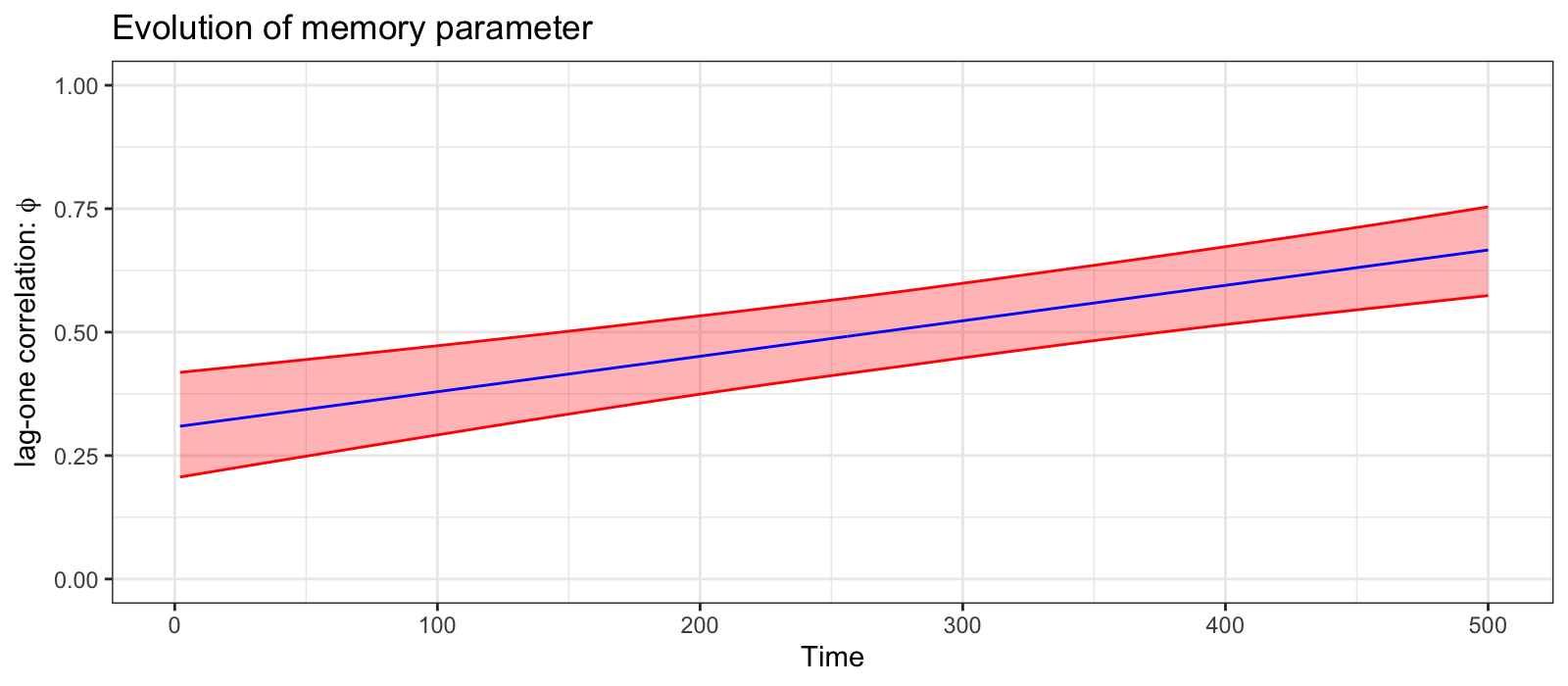
If you use this package, please cite:
- Myrvoll-Nilsen, E., Hallali, L. and Rypdal, M. (2025). Bayesian analysis of early warning signals using a time-dependent model. Earth System Dynamics, 16(5), 1539–1556. doi:10.5194/esd-16-1539-2025
@article{myrvoll2025bayesian, title = {Bayesian analysis of early warning signals using a time-dependent model}, author = {Myrvoll-Nilsen, Eirik and Hallali, Luc and Rypdal, Martin}, journal = {Earth System Dynamics}, volume = {16}, number = {5}, pages = {1539--1556}, year = {2025}, publisher = {Copernicus Publications G{\"o}ttingen, Germany}, doi = {https://doi.org/10.5194/esd-16-1539-2025} } - Hallali, L., Myrvoll-Nilsen, E. and Franzke, C. L. (2025). Assessing AMOC stability using a Bayesian nested time-dependent autoregressive model. Nonlinear Processes in Geophysics, 32(4), 383–395. doi:10.5194/npg-32-383-2025
@article{hallali2025assessing,
  title = {Assessing AMOC stability using a Bayesian nested time-dependent autoregressive model},
  author = {Hallali, Luc and Myrvoll-Nilsen, Eirik and Franzke, Christian LE},
  journal = {Nonlinear Processes in Geophysics},
  volume = {32},
  number = {4},
  pages = {383--395},
  year = {2025},
  publisher = {Copernicus GmbH},
  doi = {https://doi.org/10.5194/npg-32-383-2025}
}
Since this work is also based on other work, consider citing the following papers:
- INLA Rue, H., Martino, S. and Chopin, N. (2009). Approximate Bayesian inference for latent Gaussian models by using integrated nested Laplace approximations. Journal of the Royal Statistical Society: Series B, 71(2), 319–392. doi:10.1111/j.1467-9868.2008.00700.x
@article{rue2009, author = {Rue, H{\aa}vard and Martino, Sara and Chopin, Nicolas}, title = {Approximate {B}ayesian inference for latent {G}aussian models by using integrated nested {L}aplace approximations}, journal = {Journal of the Royal Statistical Society: Series B}, year = {2009}, volume = {71}, number = {2}, pages = {319--392}, doi = {10.1111/j.1467-9868.2008.00700.x} } - Nested AR(1) model Boers, N. (2021). Observation-based early-warning signals for a collapse of the Atlantic Meridional Overturning Circulation. Nature Climate Change, 11(8), 680–688. doi:10.1038/s41558-021-01097-4
@article{boers2021, author = {Boers, Niklas}, title = {Observation-based early-warning signals for a collapse of the {A}tlantic {M}eridional {O}verturning {C}irculation}, journal = {Nature Climate Change}, year = {2021}, volume = {11}, number = {8}, pages = {680--688}, doi = {10.1038/s41558-021-01097-4} } - Nested AR(1) model Morr, A. and Boers, N. (2024). Detection of approaching critical transitions in natural systems driven by red noise. Physical Review X, 14, 021037. doi:10.1103/PhysRevX.14.021037
@article{morr2024,
  author = {Morr, Andreas and Boers, Niklas},
  title = {Detection of approaching critical transitions in natural systems driven by red noise},
  journal = {Physical Review X},
  year = {2024},
  volume = {14},
  pages = {021037},
  doi = {10.1103/PhysRevX.14.021037}
}
- Uncertainty quantification of layer-counted data using a Bayesian regression model
- Joint synchronization of multiple chronologies using tie-points
- Scalable inference using R-INLA
The Bremla package provides a Bayesian framework for constructing and synchronizing chronologies in stratigraphic archives, with particular emphasis on layer-counted and depth-indexed records such as ice cores, sediment cores, and varved deposits. Accurate chronological inference is essential in paleoclimatology and Earth system science, as uncertainties in age models propagate directly into estimates of rates, variability, and phase relationships in paleoclimate records (McKay et al., 2021).
At its core, Bremla represents the age–depth relationship as a hierarchical Bayesian latent Gaussian model in which accumulation or deposition rates are treated as latent stochastic processes. Depth is typically observed with negligible error, while age is inferred indirectly, primarily through layer counts. This formulation yields a flexible class of models in which posterior samples of the full age–depth function can be obtained by sampling from the joint posterior distribution (Myrvoll-Nilsen et al., 2022). By exploiting Gaussian Markov random field (GMRF) structure, the resulting sparse precision matrices enable efficient computation and sampling with linear complexity in the number of depth points (Rue and Held, 2005), making the approach scalable to high-resolution datasets such as the NGRIP ice core (North Greenland Ice Core Project members, 2004).
A key extension of the framework is the incorporation of tie-points for chronology synchronization across records. These correspond to depth locations with independently constrained absolute ages and are used as probabilistic constraints within the hierarchical model. By introducing a Gaussian observation model linking predicted and observed tie-point ages, systematic biases in layer counting or deposition can be identified and corrected. This allows joint inference of synchronized chronologies while properly propagating uncertainty in both the alignment and the underlying age–depth models (Myrvoll-Nilsen et al., 2025).
Bremla leverages GMRF representations together with the R-INLA methodology (Rue et al., 2009) to enable efficient and scalable Bayesian inference for high-resolution stratigraphic models. This combination of latent Gaussian modeling and INLA-based computation provides full uncertainty quantification for age–depth relationships and synchronized chronologies, while remaining computationally tractable for large datasets. The resulting framework offers a flexible and practical tool for paleoclimate applications requiring consistent treatment of chronological uncertainty across multiple archives.
- McKay, N. P., Emile-Geay, J. and Khider, D. (2021). geoChronR – an R package to model, analyze, and visualize age-uncertain data. Geochronology, 3(1), 149–169. doi:10.5194/gchron-3-149-2021
- Myrvoll-Nilsen, E., Riechers, K. and Boers, N. (2025). Synchronization of Layer-Counted Paleoclimatic Proxy Archives Using a Bayesian Regression Modeling Framework. Bayesian Analysis, 1(1), 1–20. doi:10.1214/25-BA1509
- Myrvoll-Nilsen, E., Riechers, K., Rypdal, M. W. and Boers, N. (2022). Comprehensive uncertainty estimation of the timing of Greenland warmings in the Greenland ice core records. Climate of the Past, 18, 1275–1294. doi:10.5194/cp-18-1275-2022
- North Greenland Ice Core Project members (2004). High-resolution record of Northern Hemisphere climate extending into the last interglacial period. Nature, 431, 147–151. doi:10.1038/nature02805
- Rue, H. and Held, L. (2005). Gaussian Markov Random Fields: Theory and Applications. Chapman & Hall/CRC, Boca Raton.
- Rue, H., Martino, S. and Chopin, N. (2009). Approximate Bayesian inference for latent Gaussian models by using integrated nested Laplace approximations. Journal of the Royal Statistical Society: Series B, 71(2), 319–392. doi:10.1111/j.1467-9868.2008.00700.x
- Make sure you have R installed (https://cran.r-project.org)
- Install INLA (https://www.r-inla.org/download/)
library(remotes)
remotes::install_github('eirikmn/bremla')library(bremla)
set.seed(1)
nsims = 200 #number of chronology samples to produce
###### SIMULATE DATA ######
n=200
depth = seq(0,1,length.out=n)
dy_noise <- as.numeric(arima.sim(model=list(ar=c(0.8)),n=n,sd=sqrt(1-0.8^2)))
proxy <- as.numeric(arima.sim(model=list(ar=c(0.9)),n=n,sd=sqrt(1-0.9^2)))*5
dy <- 20*depth + proxy + dy_noise
age = cumsum(dy)
data = data.frame(age=age,dy=dy,proxy=proxy,depth=depth)
data = rbind(c(0,NA,NA,0),data) #First row is only used to extract y0 and z0.
###### MAKE TRUE AGE ######
agedisc = sin(3*pi/2/n*(1:n))*1:n/n*50
trueage = age+agedisc
###### TIE-POINTS ######
tp_ind = c(40,80,160)
tp_depths = depth[tp_ind]
tp_mean = trueage[tp_ind]
tp_std = c(1,5,25)
control.sim=list(synchronized=TRUE,
summary=list(compute=TRUE))
###### Define layer-increment model ######
formula = dy~-1+depth + proxy ## fixed effects
control.fit = list(noise='ar1', hyperprior = list( #Fit unsynchronized model
prec = list(prior='loggamma', param = c(1,0.01)),
rho = list(prior='normal', param = c(0,0.15)))
)
###### Define age-discrepancy model ######
agedisc=list(model='rw2') #uses 2nd order random walk model for age discrepancues
synchronization=list(locations=tp_depths,locations_unit='depth', #set TP depth locations
method='gauss',params=list(mean=tp_mean,sd=tp_std), #set Gaussian TP uncertainties
agedisc=agedisc
)
###### Run Bremla ######
results = bremla(formula,data,nsims=nsims,reference.label='simulated timescale',
synchronization=synchronization,
control.fit=control.fit,
control.sim=control.sim)
summary(results)
plot(results)Call:
bremla(formula, data, nsims = nsims, reference.label = 'simulated timescale', synchronization = synchronization, control.fit = control.fit, control.sim = control.sim)
Time used:
Model fitting Chron. sampling Total
3.3144 671.0021 680.2630
The fixed component is explained by linear predictor:
dy ~ -1 + depth + proxy
The noise component is explained by an ar1 process.
The model is fitted using INLA, with following estimates for the hyperparameters:
mean sd quant0.025 quant0.25 quant0.5 quant0.75 quant0.975
sigma_epsilon 0.9749 0.1021 0.7996 0.9022 0.9653 1.0383 1.1997
phi 0.7993 0.0410 0.7127 0.7727 0.8012 0.8283 0.8725
Simulating 200 chronologies, using simulated timescale as reference.
Chronologies are synchronized assuming no age discrepancy.
200 synchronized chronologies sampled using 3 tie-point distributions (Gaussian).
Tie-points are fixed at NGRIP depths (m):
0.1959799, 0.3969849, 0.798995.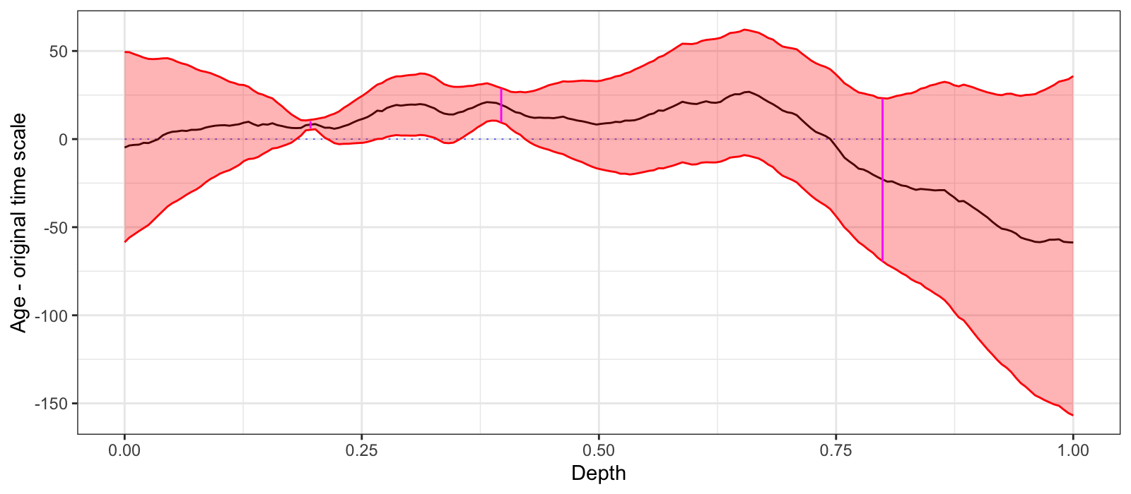
If you use this package, please cite:
- Synchronization methodology Myrvoll-Nilsen, E., Riechers, K. and Boers, N. (2025). Synchronization of Layer-Counted Paleoclimatic Proxy Archives Using a Bayesian Regression Modeling Framework. Bayesian Analysis, 1(1), 1–20. doi:10.1214/25-BA1509
@article{myrvoll2025synchronization, title = {Synchronization of Layer-Counted Paleoclimatic Proxy Archives Using a Bayesian Regression Modeling Framework}, author = {Myrvoll-Nilsen, Eirik and Riechers, Keno and Boers, Niklas}, journal = {Bayesian Analysis}, volume = {1}, number = {1}, pages = {1--20}, year = {2025}, publisher = {International Society for Bayesian Analysis}, doi = {https://doi.org/10.1214/25-BA1509} } - Bayesian regression age-depth modeling Myrvoll-Nilsen, E., Riechers, K., Rypdal, M. W. and Boers, N. (2022). Comprehensive uncertainty estimation of the timing of Greenland warmings in the Greenland ice core records. Climate of the Past, 18, 1275–1294. doi:10.5194/cp-18-1275-2022
@article{MyrvollNilsen2022,
  author = {Myrvoll-Nilsen, Eirik and Riechers, Keno and Rypdal, Martin Wibe and Boers, Niklas},
  doi = {https://doi.org/10.5194/cp-18-1275-2022},
  journal = {Climate of the Past},
  volume = {18},
  pages = {1275--1294},
  title = {Comprehensive uncertainty estimation of the timing of Greenland warmings in the Greenland ice core records},
  year = {2022}
}
Since this package use the INLA methodology, please consider citing:
- INLA Rue, H., Martino, S. and Chopin, N. (2009). Approximate Bayesian inference for latent Gaussian models by using integrated nested Laplace approximations. Journal of the Royal Statistical Society: Series B, 71(2), 319–392. doi:10.1111/j.1467-9868.2008.00700.x
@article{rue2009,
  author = {Rue, H{\aa}vard and Martino, Sara and Chopin, Nicolas},
  title = {Approximate {B}ayesian inference for latent {G}aussian models by using integrated nested {L}aplace approximations},
  journal = {Journal of the Royal Statistical Society: Series B},
  year = {2009},
  volume = {71},
  number = {2},
  pages = {319--392},
  doi = {10.1111/j.1467-9868.2008.00700.x}
}
- Models global mean surface temperature using radiative forcing and long-range dependent noise
- Supports prediction and estimation of transient climate sensitivity
- Efficient Bayesian inference using R-INLA and an approximate fractional Gaussian noise model
Quantifying the response of global mean surface temperature to radiative forcing is fundamental for assessing the risks associated with anthropogenic climate change. Statistical models used for this purpose must adequately represent both the forced response and the structure of internal climate variability.
Simple energy balance models with a single heat reservoir naturally give rise to autoregressive processes of order one (AR(1)), which are characterized by a single decorrelation timescale. However, such models fail to capture the approximately scale-invariant variability observed in empirical records of global mean surface temperature. These records exhibit long-range dependence and power-law scaling over a wide range of timescales (Rybski et al., 2006; Huybers and Curry, 2006; Franzke, 2010; Lovejoy and Schertzer, 2013; Rypdal and Rypdal, 2016). This has motivated the use of long-memory stochastic processes, such as fractional Gaussian noise (fGn), which explicitly represent persistent correlations and have been shown to provide a more realistic statistical description of temperature variability (Rypdal and Rypdal, 2016; Fredriksen and Rypdal, 2016).
A key computational challenge is that, unlike AR(1) processes, fGn is not a Gaussian Markov random field and therefore does not admit a sparse precision matrix. This makes likelihood-based inference and Bayesian computation considerably more demanding. To address this, Sørbye et al. (2019) introduced an approximation in which fGn is represented as a weighted sum of a small number of AR(1) processes. This construction recovers a sparse Markov structure, enabling efficient inference while retaining the essential long-memory properties of fGn.
The R package INLA.climate builds on these developments by providing a flexible framework for modeling the temperature response to radiative forcing within a hierarchical Bayesian setting. It leverages the R-INLA methodology (Rue et al., 2009) to perform fast and accurate approximate Bayesian inference, and incorporates the fGn approximation of Sørbye et al. (2019) to represent internal variability. This allows users to combine physically motivated response models with realistic stochastic structure, facilitating efficient estimation of key quantities such as climate sensitivity and uncertainty in the forced response across multiple timescales (Myrvoll-Nilsen et al., 2020).
In addition to model fitting, INLA.climate provides tools for prediction and climate sensitivity analysis within the same coherent Bayesian framework. In particular, it enables probabilistic projections of global mean surface temperature under user-specified future radiative forcing scenarios, allowing uncertainty in both the forced response and internal variability to be propagated forward in time. The package also facilitates estimation of key climate metrics such as the transient climate response (TCR), derived directly from the inferred model parameters. By integrating inference, prediction, and sensitivity analysis, the framework supports a comprehensive and computationally efficient approach to quantifying future climate change and its associated uncertainties.
- Franzke, C. (2010). Long-range dependence and climate noise characteristics of Antarctic temperature data. Journal of Climate, 23(22), 6074–6081. doi:10.1175/2010JCLI3654.1
- Fredriksen, H.-B. and Rypdal, K. (2016). Spectral characteristics of instrumental and climate model surface temperatures. Journal of Climate, 29(4), 1253–1268. doi:10.1175/JCLI-D-15-0457.1
- Huybers, P. and Curry, W. (2006). Links between annual, Milankovitch and continuum temperature variability. Nature, 441, 329–332. doi:10.1038/nature04745
- Lovejoy, S. and Schertzer, D. (2013). The Weather and Climate: Emergent Laws and Multifractal Cascades. Cambridge University Press.
- Myrvoll-Nilsen, E., Sørbye, S. H., Fredriksen, H.-B., Rue, H. and Rypdal, M. (2020). Statistical estimation of global surface temperature response to forcing under the assumption of temporal scaling. Earth System Dynamics, 11(2), 329–345. doi:10.5194/esd-11-329-2020
- Rue, H., Martino, S. and Chopin, N. (2009). Approximate Bayesian inference for latent Gaussian models by using integrated nested Laplace approximations. Journal of the Royal Statistical Society: Series B, 71(2), 319–392. doi:10.1111/j.1467-9868.2008.00700.x
- Rybski, D., Bunde, A., Havlin, S. and von Storch, H. (2006). Long-term persistence in climate and the detection problem. Geophysical Research Letters, 33(6), L06718. doi:10.1029/2005GL025591
- Rypdal, M. and Rypdal, K. (2016). Late Quaternary temperature variability described as abrupt transitions on a 1/f noise background. Earth System Dynamics, 7(1), 281–293. doi:10.5194/esd-7-281-2016
- Sørbye, S. H., Myrvoll-Nilsen, E. and Rue, H. (2019). An approximate fractional Gaussian noise model with $O(n)$ computational cost. Statistics and Computing, 29, 821–833. doi:10.1007/s11222-018-9843-1
- Make sure you have R installed (https://cran.r-project.org)
- Install INLA (https://www.r-inla.org/download/)
library(remotes)
remotes::install_github('eirikmn/INLA.climate')library(INLA.climate)
data(HadCRUT) #load HadCRUT GMST data
data(HansenForcingGHG) #Load Hansen et al. (2010) forcing
result <- inla.climate(data=HadCRUT$Temperature,forcing=HansenForcingGHG$Forcing,
compute.mu = 2) ## computes forcing response
summary(result)
plot(result)Call:
inla.climate(data = HadCRUT$Temperature, forcing = HansenForcingGHG$Forcing, compute.mu = 2)
Time used:
Running INLA Sampling mu Total
4.612 5.157 10.816
Random effects:
Name Model
idy RGeneric2
Model hyperparameters:
mean sd 0.025quant 0.5quant 0.975quant
H 0.8401 0.0445 0.7514 0.8407 0.9226
Sigmax 0.1316 0.0151 0.1064 0.1299 0.1655
Sigmaf 0.0647 0.0087 0.0488 0.0644 0.0828
F0 -0.1245 0.0870 -0.2951 -0.1248 0.0467
Full Bayesian analysis of forcing response computed from 100000 samples.
Deviance Information Criterion (DIC) ...: -1355.04
Effective number of parameters .........: 165.88
Marginal log-Likelihood: 898.67
Posterior marginals for linear predictor and fitted values computed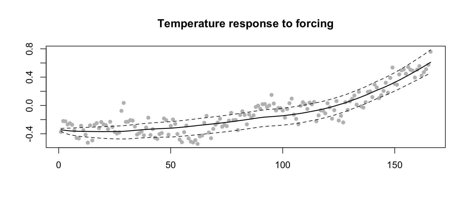
If you use this package, please cite:
- Myrvoll-Nilsen, E., Sørbye, S. H., Fredriksen, H.-B., Rue, H. and Rypdal, M. (2020). Statistical estimation of global surface temperature response to forcing under the assumption of temporal scaling. Earth System Dynamics, 11(2), 329–345. doi:10.5194/esd-11-329-2020
@article{myrvoll2020statistical,
  title = {Statistical estimation of global surface temperature response to forcing under the assumption of temporal scaling},
  author = {Myrvoll-Nilsen, Eirik and Sørbye, Sigrunn Holbek and Fredriksen, Hege-Beate and Rue, Håvard and Rypdal, Martin},
  journal = {Earth System Dynamics},
  volume = {11},
  number = {2},
  pages = {329--345},
  year = {2020},
  publisher = {Copernicus GmbH},
  doi = {https://doi.org/10.5194/esd-11-329-2020}
}
Since this package builds upon methodology from other papers, please consider citing:
- Approximate fGn model Sørbye, S. H., Myrvoll-Nilsen, E. and Rue, H. (2019). An approximate fractional Gaussian noise model with $O(n)$ computational cost. Statistics and Computing, 29, 821–833. doi:10.1007/s11222-018-9843-1
@article{Sorbye2019, author = {Sørbye, Sigrunn Holbek and Myrvoll-Nilsen, Eirik and Rue, Håvard}, title = {An approximate fractional Gaussian noise model with $O(n)$ computational cost}, journal = {Statistics and Computing}, volume = {29}, pages = {821--833}, year = {2019}, doi = {https://doi.org/10.1007/s11222-018-9843-1} } - INLA Rue, H., Martino, S. and Chopin, N. (2009). Approximate Bayesian inference for latent Gaussian models by using integrated nested Laplace approximations. Journal of the Royal Statistical Society: Series B, 71(2), 319–392. doi:10.1111/j.1467-9868.2008.00700.x
@article{rue2009,
  author = {Rue, H{\aa}vard and Martino, Sara and Chopin, Nicolas},
  title = {Approximate {B}ayesian inference for latent {G}aussian models by using integrated nested {L}aplace approximations},
  journal = {Journal of the Royal Statistical Society: Series B},
  year = {2009},
  volume = {71},
  number = {2},
  pages = {319--392},
  doi = {10.1111/j.1467-9868.2008.00700.x}
}