Bayesian age-depth modeling: Uncertainty quantification and synchronization

Background

After my PhD I started a postdoc at the Potsdam Institute for Climate Impact Research (PIK) in Germany. This position was funded by the EU Horizon 2020 program: Tipping Points in the Earth System (TiPES), and the main focus of my work was to develop a framework for quantifying dating uncertainties in layer-counted proxy records. The work evolved to also include synchronization, i.e. probabilistic alignment of multiple records using tie-points. Through this work I have collaborated closely with Niklas Boers (PIK/TUM), Keno Riechers (PIK/TUM) and Martin Rypdal (UiT).

1. Introduction

To understand the climate of the past paleoclimate proxy records are essential. These are indirect measurements of climate variables such as temperature, precipitation, or atmospheric composition, obtained from natural archives like ice cores, tree rings, sediment layers, and corals. However, these records are measured against core depth rather than time. As a result, time is therefore to be treated as an unknown latent variable and inferred from available dating information. This information is typically incorporated into age-depth models, which describes the probabilistic relationship between sediment depth and age. Proper treatment of this uncertainty is essential because it propagates through subsequent analyses and can substantially influence scientific conclusions. To account for this uncertainty, McKay et al. (CITE) recommend generating an ensemble of plausible chronologies from the age-depth model and repeating analyses across all sampled chronologies. This approach allows chronology uncertainty to be carried forward into downstream inference.

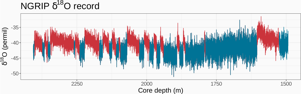
NGRIP ice core record of the oxygen isotope ratios, used as a proxy for temperature. Cold (stadial) periods are shown in blue, while warm (interstadial) periods are shown in red.

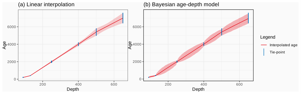
There are typically two main sources of information regarding the age-depth relationship, tie-points and layer-counts. If the archive contains dateable material at some depths, like organic matter or radioactive particles, then methods such as radiometric dating can be used to find an absolute age estimate at these depths. Using age-depth models we can interpolate these so-called tie points and obtain age-estimates of the entire core. The most simplistic age-depth models include linear or polynomial interpolation, available in packages such as CLAM (CITECITECITE). While such models are easy to use they can often provide unrealistic uncertainties. For example, we should expect the uncertainties to increase in-between observed tie-points since these depths are more uncertain. The age-depth modeling community has therefore moved towards using Bayesian age-depth models, with Bacon (CITE), BChron (CITE) and OxCal (CITE) being the most popular. These models provide robust uncertainties and can incorporate physical assumptions such as monotonicity.

Age-depth relationship inferred from tie-points, using linear interpolation with the CLAM software (a), and using the Bayesian age-depth model Bacon (b).

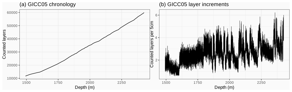
If the proxy archive is deposited in layers, for example due to seasonal variations like ice-cores and tree rings, then it is possible to obtain an age estimate by simply counting the number of layers. The number of layers counted corresponds to the number of years since 'present'. While tie-points provide an absolute age estimate, the layer-counts are instead relative to the present age. An error in the layer-count will affect every subsequent layer meaning that the uncertainties are expected to increase the further we go down in the core. Since the dating uncertainty for layer-counted records is fundamentally different from tie-point dated records we cannot adopt the same age-depth models, and there are fewer age models available for layer-counted archives. The Banded Age Model (Comboul et al., YEAR) offers a computationally efficient method, but require assumption about the underlying parameters. Boers (2018, CHECK) presents a fully Bayesian approach, but is impractical for long time series since producing chronologies from the joint posterior which respects the inferred correlation, is computationally expensive. In Myrvoll-Nilsen et al. (2022) we propose using a Bayesian regression model to describe the increments of the counted layers. By exploiting a Gaussian Markov random field structure we are able to fit the model and generate chronologies from the joint posterior in linear time.

Panel (a) shows the layer-counted chronology associated with the NGRIP ice core record, GICC05. Panel (b) shows the number of counted layers per 5cm increment.

2. Bayesian regression model

We assume that for each depth $z_k$ in the core we have a corresponding counted age $y_k$ , along with various proxies or other covariates $\bm w_k = (w_{k1},...,w_{kn_w})$ . We assume that the number of incremental layers $\Delta y_k = y_k - y_{k-1}$ in a given depth increment $\Delta z_k = z_k - <_{k-1}$ can be expressed as the sum of two components

\Delta y_k = a(\bm w_k \mid \bm \beta) + \varepsilon(z_k \mid \bm \theta) .

Here,

a(\bm w_k \mid \bm \beta) = \beta_0 + \sum_{i=1}^{n_w}\beta_i w_{ki}

denotes the structured component where the variability is explained by the measured covariates through unknown parameters $\bm \beta = (\beta_0,...,\beta_{n_w})$ , and $\varepsilon(z_k\mid \bm \theta)$ is a random effect which depend on parameters $\bm \theta = (\theta_1,...,\theta_{n_\theta})$ . In Myrvoll-Nilsen et al. (2022) we assumed $\varepsilon$ to follow an AR(1) process with parameters $\bm \theta = (\phi, \sigma)$ . The model is formulated as a latent Gaussian model and fitted using R-INLA.

The $\bm \beta$ are assigned independent vague Gaussian priors and the hyperparameters $\phi$ and $\kappa=1/\sigma^2$ are assigned the default R-INLA priors. A strong benefit with fitting the model with INLA is apparent when working with large proxy records like the NGRIP (CITECITECITE) which include over 18000 points in the pre-Holocene era. While typical simulation-based inferential methods like Markov chain Monte Carlo (MCMC) will struggle to converge, INLA is able to produce accurate approximations of the posterior marginal distributions in linear time. We can then efficiently produce samples from the fitted layer-increment model

\pi(\Delta \bm y^* \mid \Delta \bm y, \bm W) = \int \pi (\Delta \bm y^* \mid \bm \beta, \bm \theta, \bm W)\pi(\bm \beta, \bm \theta,\bm W) d\bm \beta d\bm \theta

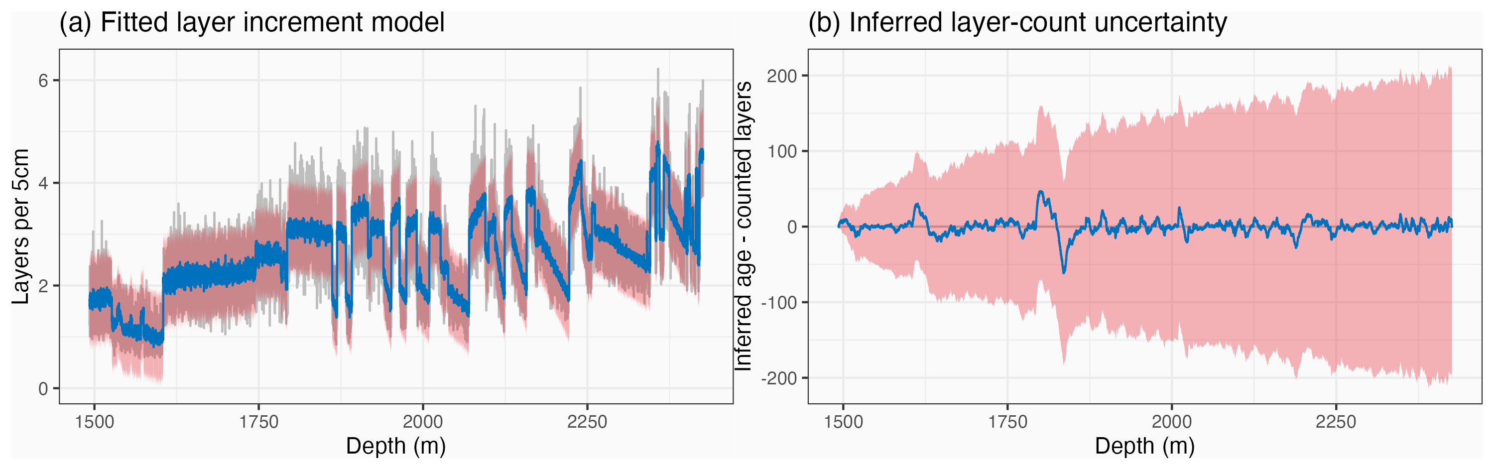
where we let $^*$ denote output from the posterior predictive distribution. By taking the cumulative sum of the sampled layer-increments $y_k^*=y_0+\sum_{i=1}^k \Delta y_i^*$ we can get sampled chronologies represented by the layer-counts.

Panel (a) shows the fitted layer-increment model with posterior mean (blue) and 95% credible intervals (red) against observed layer-increments (gray). Panel (b) shows the resulting age uncertainties obtained by taking the cumulative sums of samples from the fitted layer-increment model. The observed layer-counts for each depth has been subtracted for visibility.

3. Synchronization

If the dating uncertainty estimates are solely based on the number of counted layers, without incorporating any external information, the estimates are susceptible to potential unknown structural biases in the layer counting or accumulation process. Such biases can be revealed when comparing the estimated time scale to tie points which can be obtained by, for example, by comparing the age of known events to those of other records. This additional information could help constrain or correct age estimates, leading to improved chronologies. How to incorporate tie-points in order to meaningfully adjust the probabilistic relationship between age and core depth expressed as a joint probability distribution was an important, unsolved problem in layer-counted chronology.

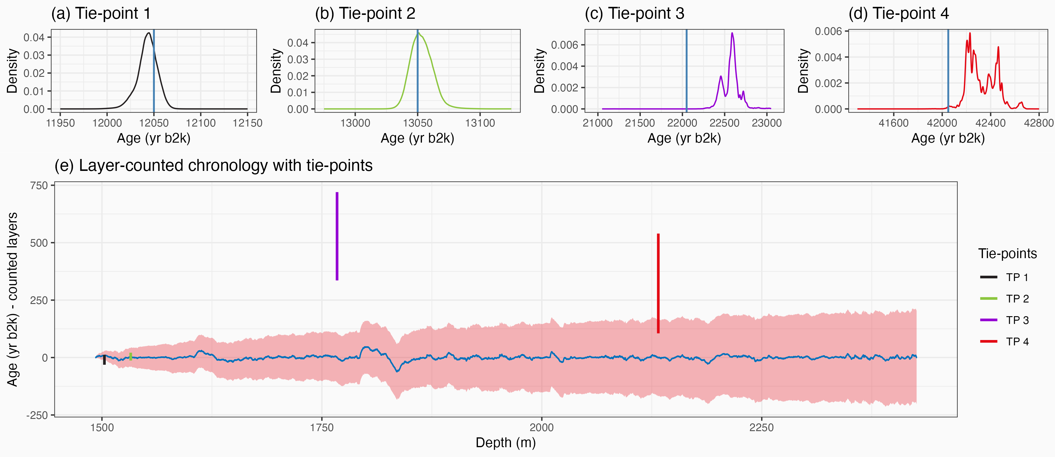
Panels (a)-(d) show tie-points obtained by Adolphi et al. (2018) and Muscheler et al. (2020). These are located at NGRIP core depths corresponding to the GICC05 ages 12050, 13050, 22050, 42050 yr b2k, respectively, illustrated by the vertical blue lines. Panel (e) shows the inferred layer-counted chronology with uncertainties, with the observed layer-counts subtracted, along with the tie-points we wish to update the chronology with.

We now have two sets of data from which we want to infer the age-depth relationship. We denote the counted layers by $\bm y_1 = (y_{1,1},...,y_{1,n})$ and the tie-points by $\bm y_2 = (y_{2,1},...,y_{2,n})$ , both observed at the full depth axis $\bm z = (z_1,...,z_n)$ . Typically, the number of observed tie-points is much smaller than the number of counted layers. Any depths which do not have an associated tie-point will be denoted by NA and is treated as a missing value.

While I described in the previous section how to infer an age-model for the layer-counts we still need to define how this relates to the new information expressed as tie-points. If there are indeed any structural biases at play which causes a discrepancy between the layer-counted age model and the true age (represented by the tie-points), then this difference needs to be accounted for as well. In Myrvoll-Nilsen et al. (2025) we add an age-discrepancy model component

\xi(z_k\mid \bm \theta) ,

which defines an appropriate model for the bias $\bm \xi = \xi(\bm z\mid \bm \theta)$ between the layer-counted chronology and the observed tie-points. In Myrvoll-Nilsen et al. (2025) we use an intrinsic second order random walk model. The layer-increment and age-discrepancy models can be fitted jointly using the linear predictor

\begin{pmatrix} \Delta \bm y_1 \\ \bm y_2 \end{pmatrix} = \begin{pmatrix} \bm I & \bm 0 \\ \bm R & \bm I \end{pmatrix}\begin{pmatrix} \Delta \bm y_1 \\ \bm \xi \end{pmatrix} ,

where

\bm R = \begin{pmatrix} \bm 1 & & \\ \vdots & \ddots & \\ 1 & \cdots& 1 \end{pmatrix}

such that $\bm y_1 = \bm R \Delta \bm y_1$ . Since $\bm R$ is not sparse this leads to a computational bottleneck. However, if we can assume that the tie-points do not affect the estimation of the layer-increments we can instead fit this model in two stages. First we fit the layer-increment model to obtain an ensemble of layer-counted chronologies $\bm y_1^*$ , then, we fit the age-discrepancy model to the differences between the tie-points and each sampled chronology. By fitting the age-discrepancy model using INLA we are able to fit each age-discrepancy model efficiently, allowing for both larger and a high number of chronology samples.

Another strength of the R-INLA that we exploit is that missing values are imputed automatically using the posterior predictive distribution inferred from the observed points. This is exactly what we want as it will generate a meaningful probabilistic interpolation between the tie-points. Samples generated from the (interpolated) posterior predictive distribution will be added to the corresponding layer-counted chronology sample, resulting in an age sample which respect both the layer-counted variability as well as the discrepancy inferred from the tie-points.

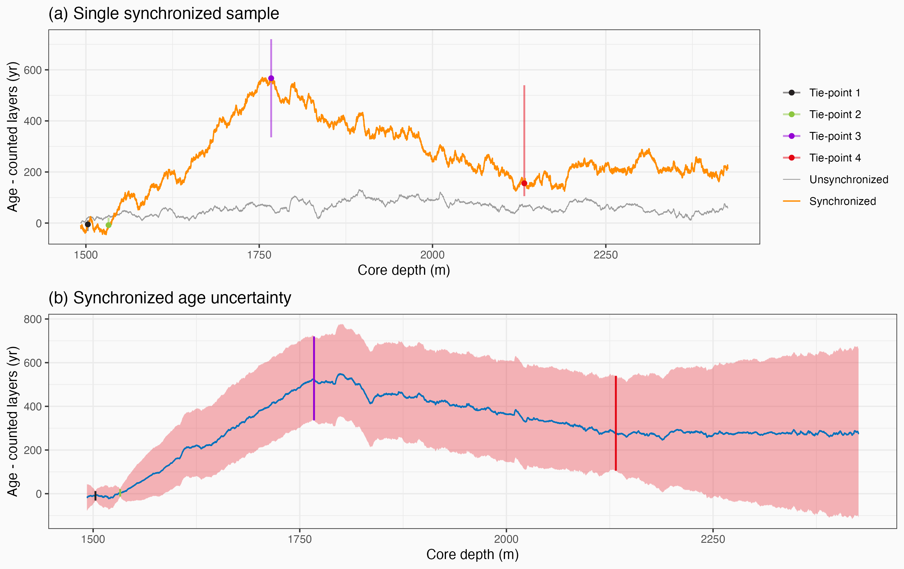
Panel (a) shows a single synchronized simulation obtained by fitting an age-discrepancy model to the difference between a single unsynchronized chronology sample and tie-points taken from the probability distribution. Panel (b) shows the synchronized age uncertainties (with the layer-counted chronology subtracted) obtained by producing an ensemble of synchronized chronology samples.

4. R-package: Bremla

The Bayesian regression modeling modeling approach to quantifying the dating uncertainties of layer-counted records, as well as the method for synchronizing chronologies to tie-points, is implemented in the 'Bremla' R-package. For more information about this package, see the Software page.