Early warning signals

Estimation of early warning signals using a Bayesian hierarchical modeling approach.

1. Background

After my postdoc position at PIK finished at the end of 2021 I returned to UiT for a 13 month position as a Researcher, funded by the TiPES project, where I worked primarily on early warning signals - statistical indicators that may precede tipping points. While the most common methods involve sliding windows we developed an alternative hierarchical Bayesian modeling approach. During this time I started supervising PhD candidate Luc Hallali whose work focused on applying these methods to Arctic climate data. Through this work I also worked with Martin Rypdal (UiT), Sigrunn Holbek Sørbye (UiT), Håvard Rue (KAUST), Christian Franzke (IBS), Clara Hummel (UiT), Alessandro Cotronei (UiT) and Niklas Boers (PIK/TUM).

2. Introduction

2.1. Tipping points and bifurcations

Many systems can undergo abrupt and sometimes irreversible transitions when critical thresholds, known as tipping points, are crossed. In climate, anthropogenic forcing has put several important components of the Earth system at risk of crossing tipping points, with potentially severe consequences for life on the planet (Armstrong McKay et al., 2022). Examples include a potential collapse of the Atlantic Meridional Overturning Circulation (AMOC; Boers, 2021), destabilization of the Greenland Ice Sheet (Boers and Rypdal, 2021) and dieback of the Amazon rainforest (Boulton et al., 2022). In order to prevent possibly irreversible changes it is crucial to know when a system is approaching a tipping point, before it is too late to course-correct.

Tipping points are naturally studied within the framework of dynamical systems, often formulated in terms of stochastic differential equations that capture the interaction between deterministic dynamics, external forcing and random fluctuations. Let, for example, $x(t)$ denote the time-dependent state variable, representing for example temperature or ice sheet volume, $dB(t)$ denote a white noise process describing the noise in the system and $F(x)$ denote the forcing of the system. The dynamical system can be expressed by

dx(t) = F(x(t)) dt + \sigma dB(t).

One could think of this equation as describing the motion of a particle in the presence of a potential $V(x)$ , with drift $F(x)=-V'(x)$ and diffusion term $\sigma dB(t)$ describing its movement. Points where $F(x)=0$ are called fixed-points. These are considered stable if a small perturbation (in any direction) near the fixed point will decay over time, and unstable otherwise. The animation below shows the potential $V(x)$ for a system with two stable fixed points (valleys), $x_1$ and $x_3$ , separated by an unstable fixed point (peak), $x_2$ . If the particle is located in the valley of an equilibrium any perturbation will be met with an opposing force pushing the particle back towards the equilibrium. If the perturbation is so large that the particle crosses the unstable fixed point separating the two domains of attraction, the particle will then be pushed towards the other stable fixed point instead. This phenomenon, where the tipping point is crossed solely from perturbations caused by the internal variation of the system, is called noise-induced tipping.

Noise-induced tipping. The dynamical system (and potential) remain unchanged. Random perturbations alone cause the system to cross the unstable fixed point (tipping point) and move into a different equilibrium.

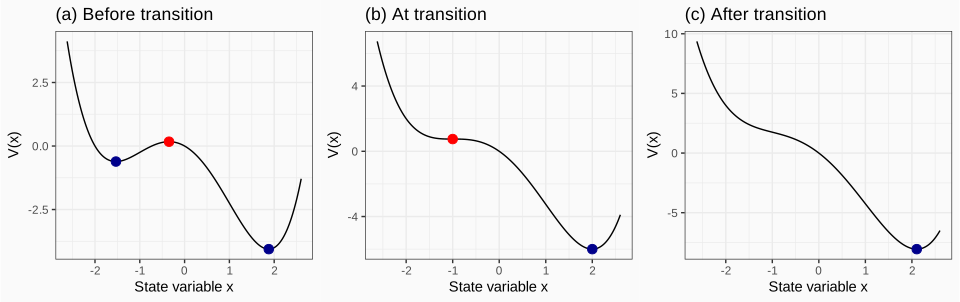
On the other hand, if the dynamics of the system depend on some slowly changing control parameter $\mu(t)$ , then fixed points may shift, vanish or spawn, depending on the value of $\mu(t)$ . This means that the stability of an equilibrium may diminish over time and eventually be lost, forcing the state variable to another equilibrium. Points where the stability or number of fixed points changes are called bifurcation points, and a critical transition caused by the control parameter approaching a bifurcation point is called a bifurcation-induced tipping process.

The potential over the state variables before (a), at (b) and after (c) the control parameter μ has reached the bifurcation point. The stable fixed points are shown in blue, while the unstable fixed points (tipping point) are shown in red. In panel (b) the unstable and first stable fixed points coincide as a single unstable saddle point.

Bifurcation-induced tipping. Gradual changes in the control parameter alter the dynamical system until a bifurcation is reached, where the left fixed point loses stability, causing the system to tip into a different equilibrium.

2.2. Critical slowing down

The nature of an equilibrium can be studied by investigating the linearization of the dynamical system around some stable fixed point $x_s$

dx(t) = -\lambda (x(t)-x_s) dt + \sigma dB(t),

where $\lambda = -F'(x_s)$ is the restoring rate. This is known as the Langevin stochastic differential equation and has the solution

x(t) = x_0 +\sigma\int_{0}^t e^{-\lambda t}dB(t) ,

which forms an Ornstein-Uhlenbeck (OU) process, and discretization yields an AR(1) process

x_t = \phi x_{t-1} + \varepsilon_t, \qquad \varepsilon_t \sim \mathcal{N}\left( 0, \frac{1-\phi^2}{2\lambda}\sigma^2 \right).

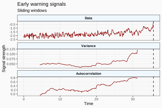
When a system approaches a bifurcation that induces destabilization, its restoring rate will decrease, causing it to recover more slowly from perturbations. This phenomenon is called critical slowing down and causes perturbations to persist for longer, leading to increased variance and autocorrelation that can serve as early warning signals of an impending critical transition (Lenton et al., 2012; Dakos et al., 2008). This phenomenon was first demonstrated by inspecting the power spectra of a simple physical model by Wiesenfeld (1985). The idea was later extended to a complex Earth system model by Held and Kleinen (2004) and first applied to real data by Dakos et al. (2008).

2.3. Sliding-window estimation

The most common approach to estimating early warning signals is to estimate each indicator in a sliding window (Boettiger and Hastings, 2012; Chen et al., 2022; Dakos et al., 2008; Dakos et al., 2012; Dakos et al., 2024; Scheffer et al., 2009), and then to use statistics like Kendall's tau to perform a hypothesis test on whether or not a statistically significant increase in the early warning signal indicators has been detected.

Sliding window estimates of the variance and autocorrelation of the observed data up to the tipping point (vertical line). Increased variance and autocorrelations suggests that the system may be approaching a bifurcation point.

While simple, sliding windows present some limitations as methods for detecting early warning signals. First, it complicates detrending, as the trends in the data can confound the estimation of the warning signals. Second, it requires a choice on the window length. Large windows offer improved stability and estimation accuracy, but assume that the underlying dynamics remain constant, which is questionable as the system approaches a bifurcation point. It will also smooth out changes, reducing the sensitivity to short-term dynamics. Smaller windows, on the other hand, will better capture the changes of the indicators, but will provide less reliable estimates, possibly leading to false positives or negatives. A good trade-off can be difficult to achieve, motivating the development of alternative methods for detecting early warning signals.

3. Model-based early warning signal detection

In Myrvoll-Nilsen et al. (2025) we circumvent sliding windows by introducing a model-based approach to early warning signals that is able to utilize the full dataset in a single, complete analysis. In short, we introduce a time-dependent AR(1) process

x_{t+1} = \phi(t) x_t + \varepsilon_{t+1}

where the lag-one autocorrelation parameter is a linear function of time

\phi(t) = a+bt , \qquad t\in (0,1) .

We assign appropriate priors on $a$ and $b$ and incorporate this into a hierarchical Bayesian model. The presence of early warning signals is then assessed by testing whether the slope parameter $b$ is positive, i.e. whether the lag-one autocorrelation is increasing over time. Being in a Bayesian framework, we are able to quantify the uncertainty of the slope parameter and assess whether it is significantly positive or not. Specifically, we say that early warning signals are detected if the posterior marginal probability of a positive slope exceeds some threshold, $1-\alpha$ , i.e.

P(b>0\mid \bm y) \geq 1-\alpha .

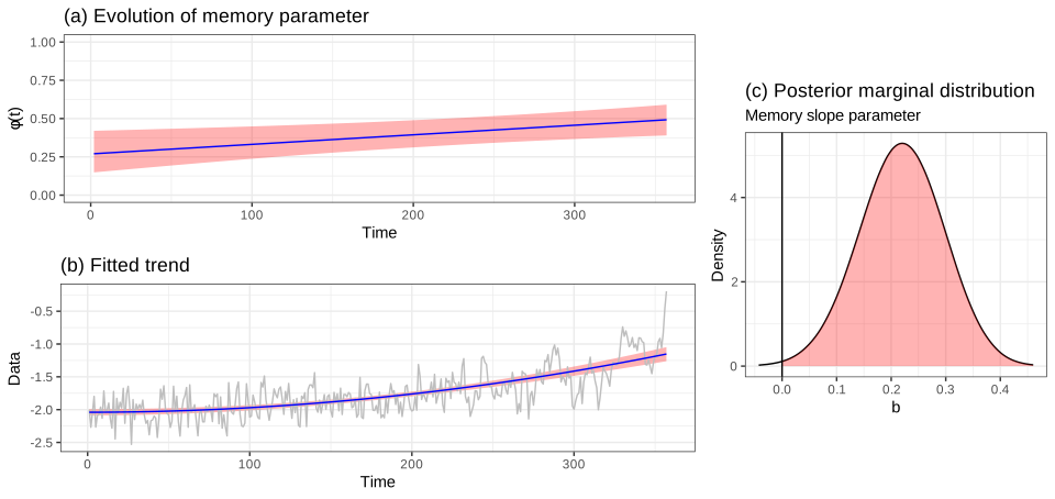
For efficient inference we adopt the R-INLA framework (Rue et al., 2009; Rue et al., 2017; r-inla.org). This ensures that the model can be fitted in a matter of seconds, even for large datasets. The following figure shows the results of applying this method to a simulated dataset with known early warning signals. The inferred evolution of the lag-one autocorrelation parameter is shown in panel (a), along with the fitted 2nd order polynomial trend in panel (b). The posterior marginal distribution of the slope parameter is shown in panel (c). In this case, we find that $P(b>0\mid \bm y) = 0.99$ , indicating that early warning signals are detected.

The inferred evolution of the time-dependent lag-one autocorrelation parameter (a), the fitted 2nd order polynomial trend (b) and the posterior marginal distribution of the memory slope parameter (c) with area above 0 shaded.

To make this method available to the wider community, we have implemented it in the R package INLA.ews. Installation instructions and a worked example, with the code and the resulting plots, are on the software page.

4. Extensions and modifications

Boers (2021) showed that using increased variance and autocorrelation as indicators for early warning signals can introduce bias, if the underlying system is driven by external noise that itself has increasing autocorrelation or variance, possibly leading to false alarms. To account for such bias, Boettner and Boers (2022) and Morr and Boers (2024) suggest that the OU process should be driven by correlated noise rather than white noise. Building upon this idea, we assume in Hallali et al. (2025) that the internal noise term is itself a time-dependent AR(1) process, leading to a nested time-dependent AR(1) process.

x_{t+1} = \phi(t) x_t + \varepsilon_{t+1}

\varepsilon_{t+1} = \rho(t) \varepsilon_t + \xi_{t+1}

Why the noise has to be modelled. Left: a system genuinely approaching a bifurcation, where the restoring rate decays and the indicators rise as a result of stability loss. Right: a system whose restoring rate never changes, driven by noise whose own autocorrelation increases over time. There is no bifurcation to approach, yet the variance and lag-one autocorrelation climb just as convincingly. The two lower rows are not distinguishable by eye, which is the difficulty the nested model is designed to resolve. 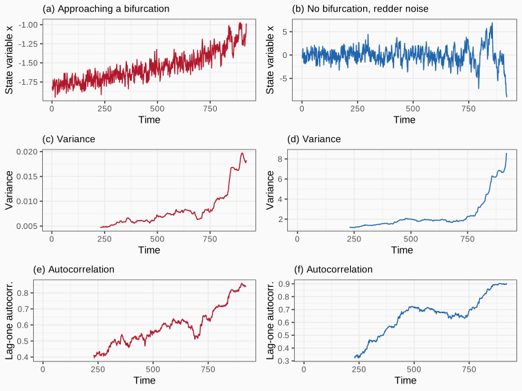— **Why the noise has to be modelled.** Left: a system genuinely approaching a bifurcation, where the restoring rate decays and the indicators rise as a result of stability loss. Right: a system whose restoring rate never changes, driven by noise whose own autocorrelation increases over time. There is no bifurcation to approach, yet the variance and lag-one autocorrelation climb just as convincingly. The two lower rows are not distinguishable by eye, which is the difficulty the nested model is designed to resolve.

where $x$ is the state variable, with stability expressed through the time-dependent autocorrelation parameter $\phi(t)$ , and $\varepsilon$ is the internal noise, which itself has time-dependent autocorrelation parameter $\rho(t)$ .

In Sørbye et al. (2026) we also extend model-based approaches to long-range dependent processes, utilizing the computationally efficient AR(1) mixture approximation of Sørbye et al. (2019), which is described in more detail in my work on long-range dependence. The time-dependent fGn model is expressed as a mixture of two fGn processes, $x_{H_1}$ and $x_{H_2}$ , with different Hurst exponents, $H_1$ and $H_2$ , where the mixture weights $w(t)$ are a linear function of time

x(t) = \sigma\left( \sqrt{1-w(t)} x_{H_1}(t)+\sqrt{w(t)}x_{H_2}(t) \right) ,

where $\sigma$ is the standard deviation. For this paper we also developed an AR(1) model where the lag-one autocorrelation parameter and the variance are not coupled through the shared parameter $\lambda$ , and are instead treated separately.

During 2025–2026 I co-supervised a Master's student on a project comparing sliding windows and model-based approaches to early warning signal detection. The results from this work suggest that sliding window approaches and model-based approaches may complement each other, as sliding window approaches could be used to help determine the appropriate model for the model-based approach.

5. Applications

5.1. Dansgaard-Oeschger events

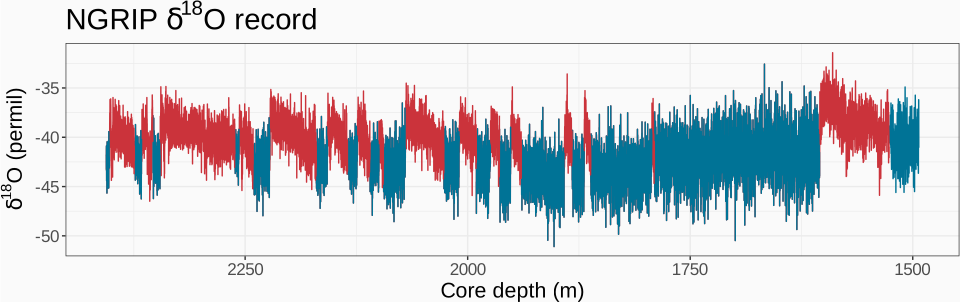
One of the first applications of the model-based approach to detect early warning signals is the Dansgaard-Oeschger (DO) events observed in Greenland ice core records. These are several critical transitions that occurred during the last ice age, where the climate changed rapidly (few decades) from a cold stadial state to a warm (up to 16 degrees warmer, locally in Greenland) interstadial state before returning gradually (over hundreds to thousands of years). These are considered by many to be the archetypal examples of climate tipping points in paleoclimate records, and whether or not these transitions are noise-induced or bifurcation-induced is contested (Ditlevsen and Johnsen, 2010; Rypdal, 2016; Boers, 2018).

NGRIP ice core record of the oxygen isotope ratios (North Greenland Ice Core Project members, 2004), used as a proxy for temperature. Cold (stadial) periods are shown in blue and warm (interstadial) periods in red, following the event stratigraphy of Rasmussen et al. (2014). The abrupt transitions from a stadial to an interstadial state are the Dansgaard–Oeschger events analysed here.

In Myrvoll-Nilsen et al. (2025) we were able to identify early warning signals for five of these transitions, using a $1-\alpha=0.95$ threshold. We revisited the same dataset in Hallali et al. (2025) using the extended model with time-dependent internal noise, and found that early warning signals were detected for six transitions. However, in Sørbye et al. (2026) we found early warning signals for none of the transitions using the fGn model, and when using the decoupled AR(1) model we identified four DO events with a significant increase in variance and one event with an increase in autocorrelation. We found no events in which both variance and autocorrelation increased simultaneously, suggesting that the coupled models may have confounded changes in variance with changes in autocorrelation.

Early warning signals detected across Dansgaard–Oeschger transitions in the NGRIP record, by model. All four analyses use the same record; the disagreement between them is the result.
Model	Study	Transitions with a signal
Time-dependent AR(1)	Myrvoll-Nilsen et al. (2025)	5
Nested time-dependent AR(1)	Hallali et al. (2025)	6
Time-dependent fGn	Sørbye et al. (2026)	none
Decoupled AR(1)	Sørbye et al. (2026)	4 variance · 1 autocorrelation · 0 both

5.2. Atlantic Meridional Overturning Circulation

Another important application of this approach is the Atlantic Meridional Overturning Circulation (AMOC). This is a large-scale ocean circulation pattern that plays a crucial role in regulating global climate. Recent studies suggest that the AMOC may be weakening (Caesar et al., 2021; Intergovernmental Panel on Climate Change, 2021) and losing resilience, potentially approaching a tipping point (Boers, 2021; Ditlevsen and Ditlevsen, 2023). An AMOC collapse would have severe consequences for the climate in Europe and North America. In Hallali et al. (2025) we applied the model-based approach to a proxy for the AMOC strength, and found that early warning signals were detected with a posterior probability of $P(b>0\mid \bm y)=0.99$ , suggesting that the AMOC may be approaching a tipping point.

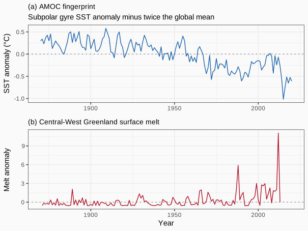
The two records behind the AMOC analysis. (a) The fingerprint of AMOC strength: the annual mean sea-surface temperature anomaly in the subpolar gyre, minus twice the global mean anomaly to compensate for polar amplification, following Caesar et al., 2018. 1870–2020. (b) Central-West Greenland surface melt Trusel et al., 2018, 1871–2013, used as forcing in one of the detrending strategies. — **The two records behind the AMOC analysis.** (a) The fingerprint of AMOC strength: the annual mean sea-surface temperature anomaly in the subpolar gyre, minus twice the global mean anomaly to compensate for polar amplification, following Caesar et al., 2018. 1870–2020. (b) Central-West Greenland surface melt Trusel et al., 2018, 1871–2013, used as forcing in one of the detrending strategies.

Since instrumental measurements only started fairly recently, a sea-surface-temperature-based proxy fingerprint of the AMOC strength is often used instead (Caesar et al., 2018; Ditlevsen and Ditlevsen, 2023). In Hallali et al. (2025) we apply both the original and the nested time-dependent AR(1) model to the fingerprint constructed by taking the annual average of the sea-surface temperature (SST) anomaly in the subpolar gyre region, minus twice the global mean SST anomaly to compensate for the polar amplification effects under global warming. The data is non-stationary, which we account for in different ways. First, we try linear and square polynomial detrending. Second, we use Central-West Greenland (CWG) surface melt (Trusel et al., 2018) as forcing. Working in the R-INLA framework allows us to fit the time-dependent model and the trends/forcing simultaneously. Using the nested AR(1) model we find statistically significant early warning signals for all detrending strategies, suggesting that the AMOC may be approaching a tipping point, and that the early warning signals are not an artifact of the detrending strategy.

5.3. The Atlantic Multidecadal Variability

The Atlantic Multidecadal Variability (AMV) is a pattern of long-term fluctuations in North Atlantic sea-surface temperatures, typically varying on timescales of about 50–80 years. It is often described as alternating periods of a warmer-than-average North Atlantic (positive AMV phase) and a cooler-than-average North Atlantic (negative AMV phase). In Sørbye et al. (2026) we applied the time-dependent fGn model to a reconstruction of the AMV provided by Michel et al. (2022), or more precisely, to a subset where the variance is approximately constant (1235--1931 CE). We find that $P(H_2-H_1>0\mid \bm y) =0.992$ , suggesting increasing autocorrelation, which is consistent with the findings of Michel et al. (2022).

6. Relevant publications

Journal article DOI PDF

A tipping point is defined by the IPCC as a critical threshold beyond which a system reorganizes, often abruptly and/or irreversibly. Tipping points can be crossed solely by internal variation in the system or by approaching a bifurcation point where the current state loses stability, which forces the system to move to another stable state. It can be shown that before a bifurcation point is reached there are observable changes in the statistical properties of the state variable. These are known as early warning signals and include increased fluctuation and autocorrelation time. It is currently debated whether or not Dansgaard–Oeschger (DO) events, which are abrupt warmings of the North Atlantic region which occurred during the last glacial period, are preceded by early warning signals. To express the changes in statistical behavior we propose a model based on the well-known first-order autoregressive (AR) process, with modifications to the autocorrelation parameter such that it depends linearly on time. In order to estimate the time evolution of the autocorrelation parameter we adopt a hierarchical Bayesian modeling framework, from which Bayesian analysis can be performed using the methodology of integrated nested Laplace approximations. We then apply the model to segments of the oxygen isotope ratios from the Northern Greenland Ice Core Project record corresponding to 17 DO events. Statistically significant early warning signals are detected for a number of DO events, which suggests that such events could indeed exhibit signs of ongoing destabilization and may have been caused by approaching a bifurcation point. The methodology developed to perform the given early warning analyses can be applied more generally and is publicly available as the R package INLA.ews.

Journal article DOI PDF

The Atlantic Meridional Overturning Circulation (AMOC) is a major climate element subject to possible ongoing loss of stability. Recent studies have found evidence of a gradual weakening in circulation, including early warning signals (EWSs), such as increased fluctuations and correlation time of the system, which are both known to be indicators of a possible forthcoming tipping point. To assess these changes in statistical behavior, we propose a robust and general statistical model based on a second-order autoregressive process with time-dependent parameters. This allows for the statistical changes from increased external variability and destabilization to be accounted for separately. We estimate the time evolution of the correlation parameters using a hierarchical Bayesian modeling framework, which also yields uncertainty quantification through the posterior distribution. To assess possible changes in AMOC stability, we apply the model to an AMOC fingerprint proxy based on the subpolar gyre and the global mean temperature anomaly. We find statistically significant EWSs, which suggests that AMOC is indeed undergoing a loss of stability and is getting closer to a tipping point. The methodology developed in this study is made publicly available as an extension of the R-package INLA.ews.

Preprint DOI PDF

Preprint.

All publications

References

Armstrong McKay, D. I., Staal, A., Abrams, J. F., Winkelmann, R., Sakschewski, B., Loriani, S., Fetzer, I., Cornell, S. E., Rockström, J. and Lenton, T. M. (2022). Exceeding 1.5\,\textdegreeC global warming could trigger multiple climate tipping points. Science, 377(6611), eabn7950. doi:10.1126/science.abn7950
Boers, N. (2018). Early-warning signals for Dansgaard–Oeschger events in a high-resolution ice core record. Nature Communications, 9, 2556. doi:10.1038/s41467-018-04881-7
Boers, N. (2021). Observation-based early-warning signals for a collapse of the Atlantic Meridional Overturning Circulation. Nature Climate Change, 11(8), 680–688. doi:10.1038/s41558-021-01097-4
Boers, N. and Rypdal, M. (2021). Critical slowing down suggests that the western Greenland Ice Sheet is close to a tipping point. Proceedings of the National Academy of Sciences, 118(21), e2024192118. doi:10.1073/pnas.2024192118
Boettiger, C. and Hastings, A. (2012). Quantifying limits to detection of early warning for critical transitions. Journal of the Royal Society Interface, 9(75), 2527–2539. doi:10.1098/rsif.2012.0125
Boettner, C. and Boers, N. (2022). Critical slowing down in dynamical systems driven by nonstationary correlated noise. Physical Review Research, 4, 013230. doi:10.1103/PhysRevResearch.4.013230
Boulton, C. A., Lenton, T. M. and Boers, N. (2022). Pronounced loss of Amazon rainforest resilience since the early 2000s. Nature Climate Change, 12, 271–278. doi:10.1038/s41558-022-01287-8
Caesar, L., McCarthy, G. D., Thornalley, D. J. R., Cahill, N. and Rahmstorf, S. (2021). Current Atlantic Meridional Overturning Circulation weakest in last millennium. Nature Geoscience, 14, 118–120. doi:10.1038/s41561-021-00699-z
Caesar, L., Rahmstorf, S., Robinson, A., Feulner, G. and Saba, V. (2018). Observed fingerprint of a weakening Atlantic Ocean overturning circulation. Nature, 556, 191–196. doi:10.1038/s41586-018-0006-5
Chen, S., Ghadami, A. and Epureanu, B. I. (2022). Practical guide to using Kendall's $\tau$ in the context of forecasting critical transitions. Royal Society Open Science, 9, 211346. doi:10.1098/rsos.211346
Dakos, V., Boulton, C. A., Buxton, J. E., Abrams, J. F., Arellano-Nava, B., Armstrong McKay, D. I., Bathiany, S., Blaschke, L., Boers, N., Dylewsky, D., López-Mart\'inez, C., Parry, I., Ritchie, P., van der Bolt, B., van der Laan, L., Weinans, E. and Kefi, S. (2024). Tipping point detection and early warnings in climate, ecological, and human systems. Earth System Dynamics, 15(4), 1117–1135. doi:10.5194/esd-15-1117-2024
Dakos, V., Carpenter, S. R., Brock, W. A., Ellison, A. M., Guttal, V., Ives, A. R., Kéfi, S., Livina, V., Seekell, D. A., van Nes, E. H. and Scheffer, M. (2012). Methods for detecting early warnings of critical transitions in time series illustrated using simulated ecological data. PLoS ONE, 7(7), e41010. doi:10.1371/journal.pone.0041010
Dakos, V., Scheffer, M., van Nes, E. H., Brovkin, V., Petoukhov, V. and Held, H. (2008). Slowing down as an early warning signal for abrupt climate change. Proceedings of the National Academy of Sciences, 105(38), 14308–14312. doi:10.1073/pnas.0802430105
Ditlevsen, P. and Ditlevsen, S. (2023). Warning of a forthcoming collapse of the Atlantic meridional overturning circulation. Nature Communications, 14(1), 4254. doi:10.1038/s41467-023-39810-w
Ditlevsen, P. D. and Johnsen, S. J. (2010). Tipping points: Early warning and wishful thinking. Geophysical Research Letters, 37(19), L19703. doi:10.1029/2010GL044486
Hallali, L., Myrvoll-Nilsen, E. and Franzke, C. L. (2025). Assessing AMOC stability using a Bayesian nested time-dependent autoregressive model. Nonlinear Processes in Geophysics, 32(4), 383–395. doi:10.5194/npg-32-383-2025
Held, H. and Kleinen, T. (2004). Detection of climate system bifurcations by degenerate fingerprinting. Geophysical Research Letters, 31(23), L23207. doi:10.1029/2004GL020972
Intergovernmental Panel on Climate Change (2021). Climate Change 2021: The Physical Science Basis. Contribution of Working Group I to the Sixth Assessment Report. Cambridge University Press. doi:10.1017/9781009157896
Lenton, T. M., Livina, V. N., Dakos, V., van Nes, E. H. and Scheffer, M. (2012). Early warning of climate tipping points from critical slowing down: comparing methods to improve robustness. Philosophical Transactions of the Royal Society A, 370(1962), 1185–1204. doi:10.1098/rsta.2011.0304
Michel, S. L. L., Swingedouw, D., Ortega, P., Gastineau, G., Mignot, J., McCarthy, G. and Khodri, M. (2022). Early warning signal for a tipping point suggested by a millennial Atlantic Multidecadal Variability reconstruction. Nature Communications, 13, 5176. doi:10.1038/s41467-022-32704-3
Morr, A. and Boers, N. (2024). Detection of approaching critical transitions in natural systems driven by red noise. Physical Review X, 14, 021037. doi:10.1103/PhysRevX.14.021037
Myrvoll-Nilsen, E., Hallali, L. and Rypdal, M. (2025). Bayesian analysis of early warning signals using a time-dependent model. Earth System Dynamics, 16(5), 1539–1556. doi:10.5194/esd-16-1539-2025
North Greenland Ice Core Project members (2004). High-resolution record of Northern Hemisphere climate extending into the last interglacial period. Nature, 431, 147–151. doi:10.1038/nature02805
Rasmussen, S. O., Bigler, M., Blockley, S. P., Blunier, T., Buchardt, S. L., Clausen, H. B., Cvijanovic, I., Dahl-Jensen, D., Johnsen, S. J., Fischer, H., Gkinis, V., Guillevic, M., Hoek, W. Z., Lowe, J. J., Pedro, J. B., Popp, T., Seierstad, I. K., Steffensen, J. P., Svensson, A. M., Vallelonga, P., Vinther, B. M., Walker, M. J. C., Wheatley, J. J. and Winstrup, M. (2014). A stratigraphic framework for abrupt climatic changes during the Last Glacial period based on three synchronized Greenland ice-core records: refining and extending the INTIMATE event stratigraphy. Quaternary Science Reviews, 106, 14–28. doi:10.1016/j.quascirev.2014.09.007
Rue, H., Martino, S. and Chopin, N. (2009). Approximate Bayesian inference for latent Gaussian models by using integrated nested Laplace approximations. Journal of the Royal Statistical Society: Series B, 71(2), 319–392. doi:10.1111/j.1467-9868.2008.00700.x
Rue, H., Riebler, A., Sørbye, S. H., Illian, J. B., Simpson, D. P. and Lindgren, F. K. (2017). Bayesian computing with INLA: a review. Annual Review of Statistics and Its Application, 4, 395–421. doi:10.1146/annurev-statistics-060116-054045
Rypdal, M. (2016). Early-warning signals for the onsets of Greenland interstadials and the Younger Dryas–Preboreal transition. Journal of Climate, 29(11), 4047–4056. doi:10.1175/JCLI-D-15-0828.1
Scheffer, M., Bascompte, J., Brock, W. A., Brovkin, V., Carpenter, S. R., Dakos, V., Held, H., van Nes, E. H., Rietkerk, M. and Sugihara, G. (2009). Early-warning signals for critical transitions. Nature, 461(7260), 53–59. doi:10.1038/nature08227
Sørbye, S. H., Myrvoll-Nilsen, E. and Rue, H. (2019). An approximate fractional Gaussian noise model with $O(n)$ computational cost. Statistics and Computing, 29, 821–833. doi:10.1007/s11222-018-9843-1
Sørbye, S. H., Myrvoll-Nilsen, E. and Rue, H. (2026). Bayesian identification of early warning signals for long-range dependent climatic time series. arXiv. doi:10.48550/arXiv.2602.09731
Trusel, L. D., Das, S. B., Osman, M. B., Evans, M. J., Smith, B. E., Fettweis, X., McConnell, J. R., No\"el, B. P. Y. and van den Broeke, M. R. (2018). Nonlinear rise in Greenland runoff in response to post-industrial Arctic warming. Nature, 564, 104–108. doi:10.1038/s41586-018-0752-4
Wiesenfeld, K. (1985). Noisy precursors of nonlinear instabilities. Journal of Statistical Physics, 38, 1071–1097. doi:10.1007/BF01010430