By approximating a long-range dependent process using a mixture of four AR(1) processes we are able to achieve efficient and accurate Bayesian inference. This methodology was used to model global mean surface temperature.
1. Background
After finishing my master's thesis at NTNU in September 2016, I started my PhD at UiT The Arctic University of Norway, under the supervision of Sigrunn Holbek Sørbye (UiT), and co-supervision of Håvard Rue (KAUST) and Martin Rypdal (UiT). The main aim of my PhD thesis was to develop an efficient approximation of long-memory processes that allows for fast Bayesian inference, and to use this methodology to analyze global mean surface temperature records. In addition to my supervisors, I also collaborated with Hege-Beate Fredriksen (UiT) and Kristoffer Rypdal (UiT).
2. Introduction
2.1. Fractional Gaussian noise
Long-range dependence (LRD) or long memory is a property relating to the rate of decay of statistical dependence of two observations as the distance between them increases. A common definition for long-memory behavior is given by a hyperbolic (as opposed to an exponential) decay of the autocovariance function.
Cov(Xt,Xt+k)∼k2H−2.
Here, H measures the degree of long-range dependence and is commonly referred to as the Hurst exponent. The exponent is named after H.E. Hurst, who, while studying the storage requirements of reservoirs on the Nile River, observed that the rescaled range statistic of hydrological records followed a power-law (Hurst, 1951), which could not be explained using contemporary short memory models. Hurst's results led to increased interest in the topic, and both hydrologists and mathematicians tried to find theoretical explanations of the so-called Hurst phenomenon.
A major breakthrough came with the introduction of fractional Brownian motion and its increment process, fractional Gaussian noise (fGn), by Mandelbrot and van Ness (1968). This is a process with an autocovariance function that decays hyperbolically
It can be shown (see e.g. Theorem 2.2 in Rue and Held, 2005) that if two variables xi and xj, in a Gaussian random field x, are conditionally independent given the other variables in the field, x−ij, the corresponding term in the precision matrix is zero, i.e. Qij=0. Thus, if x has a high degree of conditional independence we say that it is a Gaussian Markov random field (GMRF) and the precision matrix (inverse covariance matrix) will then be sparse. For example, since each node of an AR(1) process is only conditionally dependent on its immediate predecessor it is a GMRF with a tridiagonal precision matrix.
Conditional dependence structure for an AR(1) process. Each node only depends (directly) on its immediate predecessor. This Markov property ensures a sparse precision matrix which allows for the use of computationally efficient algorithms.
The sparse precision matrix associated with the Markov property allows for many efficient algorithms for key operations to be utilized. This includes computing the log-likelihood (Rue, 2001), performing Cholesky factorization and producing samples. This is particularly important for Bayesian inference, where the posterior distributions are typically evaluated using time-consuming sampling-based methods such as Markov chain Monte Carlo (MCMC). The Markov property allows for these methods to be implemented more efficiently, but also allows for more efficient alternatives such as integrated nested Laplace approximations (INLA, Rue et al., 2009). INLA utilizes the sparse structure of the precision matrix to compute the posterior marginal distributions numerically, foregoing the need for sampling.
Unlike Markov processes like the AR(1), long-memory processes exhibit persistent correlations over extended time periods, where each variable is conditionally dependent on all other variables. This means that the precision matrix is dense, and key inference algorithms have a computational cost that scales cubically with the number of observations, making them impractical for large datasets. In simple cases it is possible to exploit the Toeplitz structure of the covariance matrix to achieve O(n2) cost, but in many situations, such as when we have inhomogeneous variance, the Toeplitz structure breaks and the cost increases to O(n3). This motivates the need for an approximate model that can capture the long range dependence of the fGn process while retaining the Markov property, allowing for efficient inference algorithms to be utilized.
Conditional dependence structure for an fGn process. All nodes have a direct dependence with all other nodes. This makes inference, and many important matrix operations, computationally expensive.
Granger (1980) showed that if the lag-one autocorrelation parameter ϕ of an AR(1) process is sampled from a beta distribution the aggregation of AR(1) processes would exhibit long-range dependence according to a fractionally integrated process. It should therefore, in theory, be possible to express an fGn process through a mixture of short memory processes, which would grant the Markov property and possibly reduce computational cost.
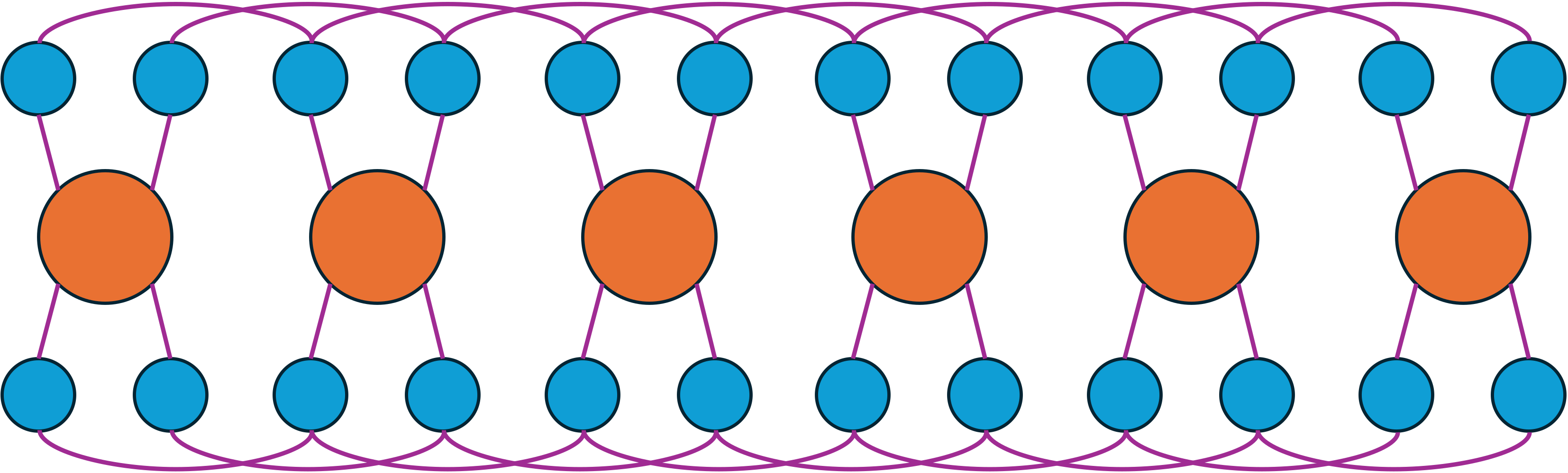
Conditional dependence structure for an approximate fGn process, expressed as a mixture of four AR(1) processes. The dependency between different nodes of the fGn process (orange) is expressed only through the individual AR(1) processes (blue). This makes the approximate model inherit the Markov property, allowing for efficient inference.
Unfortunately, as pointed out by Haldrup and Vera-Valdés (2017), the number of AR(1) processes (with ϕ drawn from a beta distribution) required to exhibit long-range dependence is so large that any gains in the Markov property would be lost to the increase in variables associated with the high number of AR(1) processes, making a sampling-based approach impractical for inference.
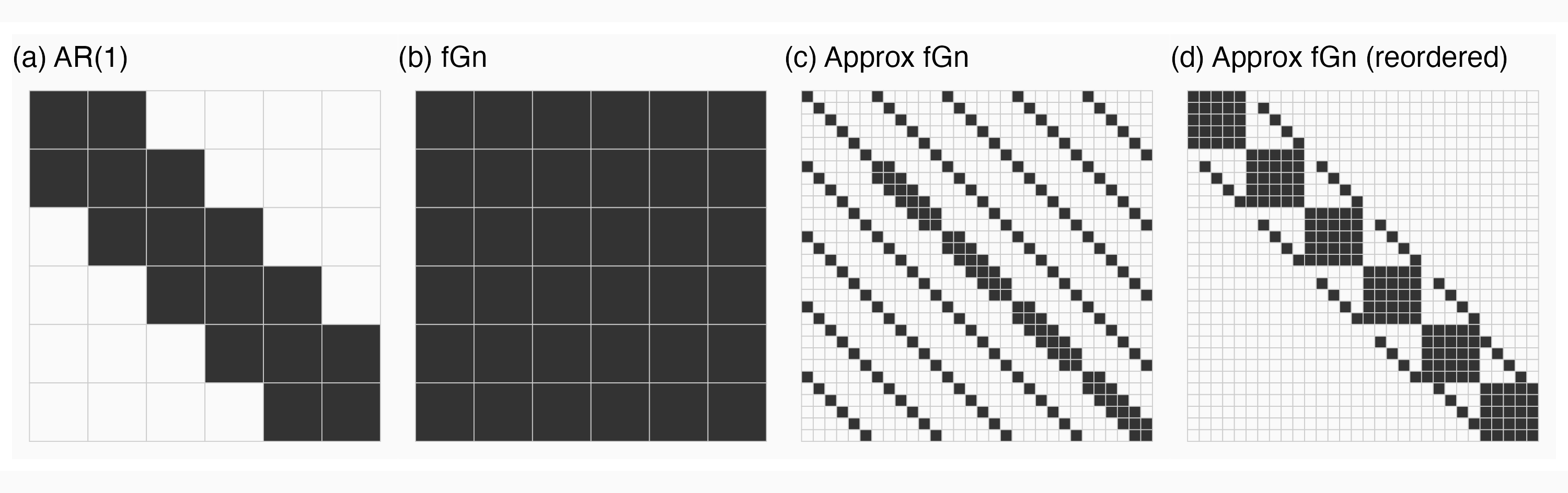
Sparsity pattern of the precision matrix of (a) an AR(1) process, (b) an fGn process and (c) an approximate fGn as a mixture of 4 AR(1) processes. In (d), the AR(1) mixture process has been reordered such that the precision matrix becomes a band matrix.
3. AR(1) mixture approximation
In Sørbye et al. (2019) we propose a numerical approach to approximating long-range dependence by aggregating AR(1) processes. Specifically, we approximate the fGn process z by:
z~=i=1∑mwixi+τ
where xi denote independent AR(1) processes with unit variance and lag-one correlation ϕi. To avoid a singular precision matrix for the joint GMRF (z~,x1,...,xm) we add a small noise term τ∼N(0,exp(−15)). Instead of drawing the lag-one parameters from a random distribution we instead used numerical optimization to find the weights w and lag-one parameters ϕ which results in the autocorrelation function (acf), γz~, which (up to a selected lag kmax) best approximates the target acf, γH, of an fGn with some Hurst exponent H,
γz~(k)=i=1∑mwiϕik.
Formally, the optimization problem can be expressed as:
(w,ϕ)H=w,ϕargmink=1∑kmaxk1(γz~(k)−γH(k))2
and is repeated for all H in a grid covering the persistent range, H∈(0.5,1). The weighting term 1/k is used to give more importance to small lags in the optimization procedure, which are more important for estimation accuracy. The optimization yields a mapping from H to a corresponding set of weights w and lag-one autocorrelation parameters ϕ, which in turn gives us an approximate fGn process expressed as a mixture of m AR(1) processes. We find that only using m=4 AR(1) processes in the aggregation provides excellent approximation of the autocorrelation function. We also find good estimation accuracy even for time series exceeding kmax=1000. See Sørbye et al. (2019) or Myrvoll-Nilsen (2020) for more details.
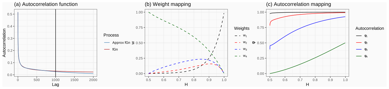
Panel (a) shows the autocorrelation function of an approximate fGn process, using 4 AR(1) processes, against the correlation function of a target fGn process with H = 0.8. The mapping from each H in the persistent range of (0.5, 1) to the corresponding weights and lag-one autocorrelation parameters are shown in panels (b) and (c), respectively.
To fully exploit the computational advantages of a GMRF approximation of an fGn we formulate a latent Gaussian model, and perform full Bayesian inference using INLA through its implementation in R (r-inla.org). Being able to incorporate the model into the R-INLA framework allows us to easily add other model components such as seasonal trends and random effects. The model has since been incorporated into R-INLA as a standard model.
The approximate fGn model laid the foundation for my PhD thesis, and was subsequently applied to a number of real-world problems in climate science.
To understand how radiative forcing affects the GMST we can use a simple energy balance model, which describes the change in heat content of the climate system as a function of the radiative forcing F and the heat loss to space. This can be expressed as
dtdΔQ=−λΔT+F
and ΔQ=CΔT, where ΔQ is the change in the system's heat content, C is the heat capacity, ΔT is the temperature anomaly and λ is the feedback parameter. The forcing can be decomposed into a known component Fknown, and an unknown, stochastic component dB(t). By solving the energy balance model we find that the GMST can be expressed as the sum of two components. First, the response to known forcing
μ(t)=C1∫0tg(t−s)Fknown(s)ds
where g(t−s)=e−(t−s)λ/C is the Green's function. And second, an Ornstein-Uhlenbeck process ε which describes the response to the stochastic forcing component
ε(t)=Cσ∫0tg(t−s)dB(s).
When discretized, the stochastic component results in an AR(1) process. This model is, however, not consistent with observations (Rypdal and Rypdal, 2014) due to the slow climate response associated with the energy exchange with the deep ocean. This simple energy balance model can be extended to an m-box model where heat is exchanged between m 'boxes', representing different layers of the deep ocean. Mathematically, the m-box model can be expressed as
CdtdΔT(t)=KΔT(t)+F(t).
Here, K is a matrix representing the heat exchange between the boxes. As the number of boxes increases towards infinity, the Green's function can be expressed as a scale invariant response function (Fredriksen and Rypdal, 2017)
g(t)=tH−3/2,
which means that the response to the stochastic component can be expressed as a fractional Gaussian noise process with Hurst exponent H. Moreover, letting F0 denote an unknown shift parameter in the known forcing, and σ and σf be scaling parameters for the stochastic and known forcing, respectively, we can express the GMST as
ΔT=μ(H,F0,σf)+ε(H,σ).
Since none of the default R-INLA models support this specific formulation we need to construct the latent model component using the custom modeling framework of R-INLA called rgeneric. To make the temperature response model easily accessible to other researchers we have developed a user-friendly R-package called INLA.climate, which takes care of the technical implementation of the model and allows users to easily fit the model to their data using R-INLA. This package is available at my GitHub repository: INLA.climate, and a demonstration and short description is also available under the 'Software' section of this website. A more detailed description and tutorial of this package can be found in Appendix A in my PhD thesis (Myrvoll-Nilsen, 2020).
5. Climate applications
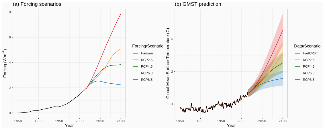
There are several benefits of having the model specified through the R-INLA framework. For example, any missing values in the GMST will be imputed automatically using the posterior predictive distribution (but the known forcing has to be provided as input for all points). This also means that we can very easily use the model for prediction. In Myrvoll-Nilsen et al. (2020) we predict the GMST under the four Representation Concentration Pathways (RCP) provided by the Coupled Model Intercomparison Project (CMIP) for the period 2006-2100, and find that the model provides good predictive performance even for long-term predictions up to 100 years into the future.
Panel (a) shows the Hansen Greenhouse Gas forcing extended with the four RCP scenarios. Panel (b) shows the HadCRUT global mean surface temperature with predicted posterior marginal mean and 95% credible intervals for each RCP scenario.
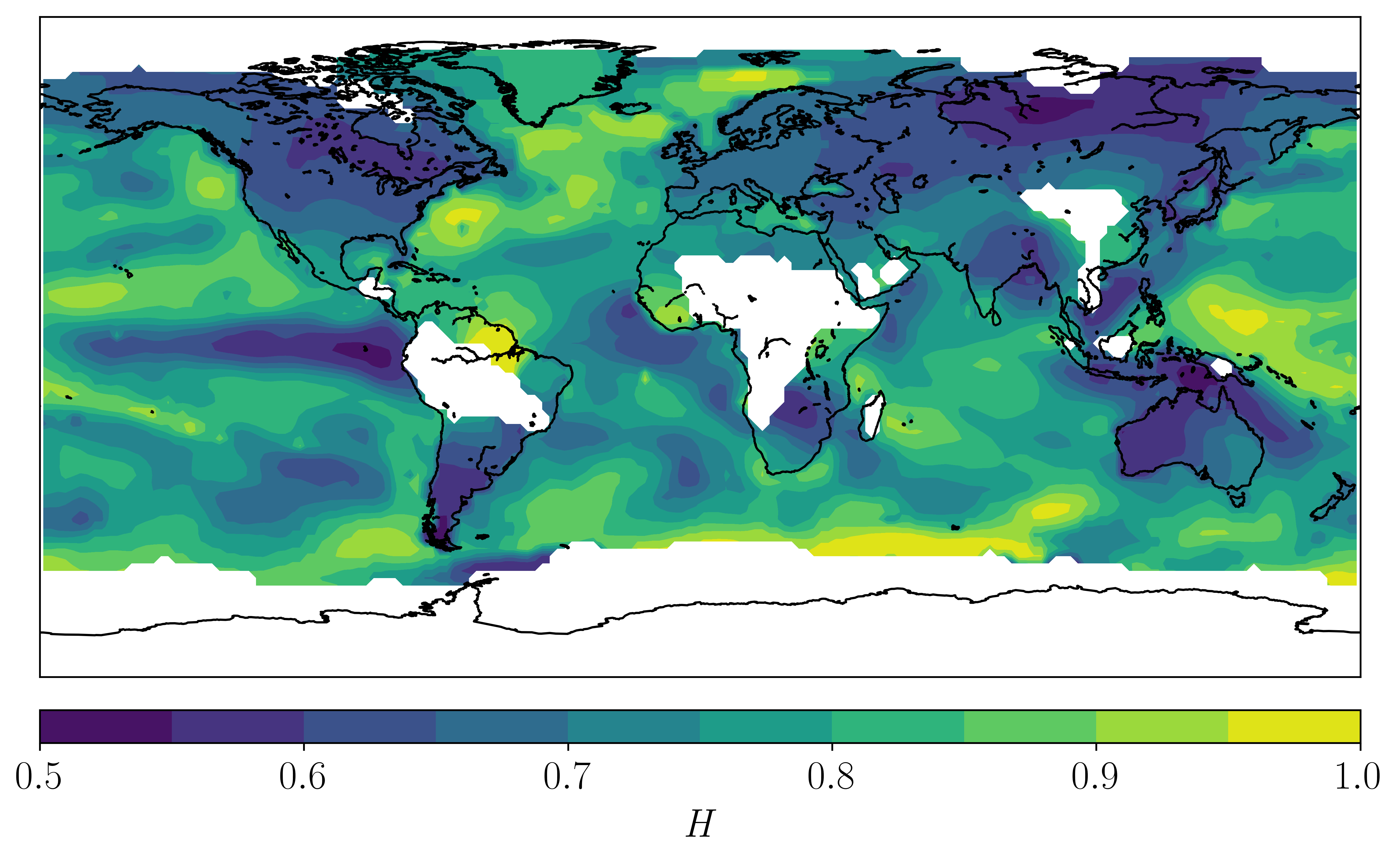
In other applications we use the model to estimate both the transient climate sensitivity (Myrvoll-Nilsen et al., 2020) and the equilibrium climate sensitivity (Rypdal et al., 2018), which are key metrics for understanding the risk of dangerous anthropogenic climate change. In Myrvoll-Nilsen et al. (2019) we exploit the reduced computational cost in order to fit the model to all local temperature records in the spatio-temporal dataset, GISS Surface Temperature Analysis version 4 (GISTEMP v4) (GISTEMP Team, 2018; Lenssen et al., 2019).
Image taken from Myrvoll-Nilsen et al. (2019). The posterior marginal mean estimate of the Hurst exponent obtained from fitting an fGn model using global radiative forcing to local time series data from the GISTEMP v4 spatio-temporal temperature dataset, for the years 1900–2015.
6. Relevant publications in this field
Emergent scale invariance and climate sensitivity
Rypdal, Martin and Fredriksen, Hege-Beate and Myrvoll-Nilsen, Eirik and Rypdal, Kristoffer and Sørbye, Sigrunn H
Earth’s global surface temperature shows variability on an extended range of temporal scales and satisfies an emergent scaling symmetry. Recent studies indicate that scale invariance is not only a feature of the observed temperature fluctuations, but an inherent property of the temperature response to radiative forcing, and a principle that links the fast and slow climate responses. It provides a bridge between the decadal- and centennial-scale fluctuations in the instrumental temperature record, and the millennial-scale equilibration following perturbations in the radiative balance. In particular, the emergent scale invariance makes it possible to infer equilibrium climate sensitivity (ECS) from the observed relation between radiative forcing and global temperature in the instrumental era. This is verified in ensembles of Earth system models (ESMs), where the inferred values of ECS correlate strongly to estimates from idealized model runs. For the range of forcing data explored in this paper, the method gives best estimates of ECS between 1.8 and 3.7 K, but statistical uncertainties in the best estimates themselves will provide a wider likely range of the ECS.
An approximate fractional Gaussian noise model with O(n) computational cost
Sørbye, Sigrunn Holbek and Myrvoll-Nilsen, Eirik and Rue, Håvard
Fractional Gaussian noise (fGn) is a stationary time series model with long-memory properties applied in various fields like econometrics, hydrology and climatology. The computational cost in fitting an fGn model of length n using a likelihood-based approach is O(n2), exploiting the Toeplitz structure of the covariance matrix. In most realistic cases, we do not observe the fGn process directly but only through indirect Gaussian observations, so the Toeplitz structure is easily lost and the computational cost increases to O(n3). This paper presents an approximate fGn model of O(n) computational cost, both with direct and indirect Gaussian observations, with or without conditioning. This is achieved by approximating fGn with a weighted sum of independent first-order autoregressive (AR) processes, fitting the parameters of the approximation to match the autocorrelation function of the fGn model. The resulting approximation is stationary despite being Markov and gives a remarkably accurate fit using only four AR components. Specifically, the given approximate fGn model is incorporated within the class of latent Gaussian models in which Bayesian inference is obtained using the methodology of integrated nested Laplace approximation. The performance of the approximate fGn model is demonstrated in simulations and two real data examples.
Warming trends and long-range dependent climate variability since year 1900: A Bayesian approach
Myrvoll-Nilsen, Eirik and Fredriksen, Hege-Beate and Sørbye, Sigrunn H and Rypdal, Martin
Temporal persistence in unforced climate variability makes detection of trends in surface temperature difficult. Part of the challenge is methodological since standard techniques assume a separation of time scales between trend and noise. In this work we present a novel Bayesian approach to trend detection under the assumption of long-range dependent natural variability, and we use estimates of historical forcing to test if the method correctly discriminates trends from low-frequency natural variability. As an application we analyze 2° × 2° gridded data from the GISS Surface Temperature Analysis. In the time period from 1900 to 2015 we find positive trends for 99% of the grid points. For 84% of the grid points we are confident that the trend is positive, meaning that the 95% credibility interval for the temperature trend contained only positive values. This number increased to 89% when we used estimates of historical forcing to specify the noise model. For the time period from 1900 to 1985 the corresponding ratios were 42 and 52%. Our findings demonstrate that positive trends since 1900 are now detectable locally over most of Earth's surface.
Statistical estimation of global surface temperature response to forcing under the assumption of temporal scaling
Myrvoll-Nilsen, Eirik and Sørbye, Sigrunn Holbek and Fredriksen, Hege-Beate and Rue, Håvard and Rypdal, Martin
Reliable quantification of the global mean surface temperature (GMST) response to radiative forcing is essential for assessing the risk of dangerous anthropogenic climate change. We present the statistical foundations for an observation-based approach using a stochastic linear response model that is consistent with the long-range temporal dependence observed in global temperature variability. We have incorporated the model in a latent Gaussian modeling framework, which allows for the use of integrated nested Laplace approximations (INLAs) to perform full Bayesian analysis. As examples of applications, we estimate the GMST response to forcing from historical data and compute temperature trajectories under the Representative Concentration Pathways (RCPs) for future greenhouse gas forcing. For historic runs in the Model Intercomparison Project Phase 5 (CMIP5) ensemble, we estimate response functions and demonstrate that one can infer the transient climate response (TCR) from the instrumental temperature record. We illustrate the effect of long-range dependence by comparing the results with those obtained from one-box and two-box energy balance models. The software developed to perform the given analyses is publicly available as the R package INLA.climate.
Efficient Bayesian analysis of long memory processes applied to climate
Temperature fluctuations can be described by a persistent correlation structure known as long-range dependence (LRD). This is a phenomenon which implies that the autocorrelation function follows a power-law decay and that observations may still be significantly correlated even if the temporal or spatial distance between them is large. Moreover, temperature is known to be influenced by radiative forcing, or how much of the solar radiation is absorbed by the earth. This is affected by factors such as solar variation and emission of climate gases. The topic of this thesis is to develop efficient statistical methodology to obtain Bayesian inference for global and local climatic time series data. This is achieved using the general hierarchical modeling framework of latent Gaussian models. Bayesian analysis can be performed efficiently using the methodology of integrated nested Laplace approximation (INLA), utilising the sparse structure of the inverse covariance matrix of the latent Gaussian field. Obtaining inference for LRD processes using INLA is inefficient on account of their dense inverse covariance matrix. Paper I demonstrates how stationary Gaussian LRD processes with memory governed by a single-parameter can be approximated with great accuracy using a mixture of four first-order autoregressive processes. This approximation ensures that the LRD model retains conditional independence and that inference can be obtained in linear time and memory. Paper II details how this methodology can be used to design a Bayesian model for global mean surface temperature (GMST) that reflects climate dynamics by incorporating radiative forcing data. This model is available as the R-package INLA.climate and is used to estimate the transient climate response and to predict temperature response to future forcing scenarios. Paper III uses the GMST model to estimate equilibrium climate sensitivity, and paper IV applies the same methodology to gridded local time series.
Franzke, C. (2010). Long-range dependence and climate noise characteristics of Antarctic temperature data. Journal of Climate, 23(22), 6074–6081. doi:10.1175/2010JCLI3654.1
Fredriksen, H.-B. and Rypdal, K. (2016). Spectral characteristics of instrumental and climate model surface temperatures. Journal of Climate, 29(4), 1253–1268. doi:10.1175/JCLI-D-15-0457.1
Fredriksen, H.-B. and Rypdal, M. (2017). Long-range persistence in global surface temperatures explained by linear multibox energy balance models. Journal of Climate, 30(18), 7157–7168. doi:10.1175/JCLI-D-16-0877.1
GISTEMP Team (2018). GISS Surface Temperature Analysis (GISTEMP). NASA Goddard Institute for Space Studies. data.giss.nasa.gov/gistemp/
Granger, C. W. J. (1980). Long memory relationships and the aggregation of dynamic models. Journal of Econometrics, 14(2), 227–238. doi:10.1016/0304-4076(80)90092-5
Haldrup, N. and Vera-Valdés, J. E. (2017). Long memory, fractional integration, and cross-sectional aggregation. Journal of Econometrics, 199(1), 1–11. doi:10.1016/j.jeconom.2017.03.001
Hurst, H. E. (1951). Long-term storage capacity of reservoirs. Transactions of the American Society of Civil Engineers, 116, 770–799. doi:10.1061/TACEAT.0006518
Huybers, P. and Curry, W. (2006). Links between annual, Milankovitch and continuum temperature variability. Nature, 441, 329–332. doi:10.1038/nature04745
Lenssen, N. J. L., Schmidt, G. A., Hansen, J. E., Menne, M. J., Persin, A., Ruedy, R. and Zyss, D. (2019). Improvements in the GISTEMP uncertainty model. Journal of Geophysical Research: Atmospheres, 124(12), 6307–6326. doi:10.1029/2018JD029522
Lovejoy, S. and Schertzer, D. (2013). The Weather and Climate: Emergent Laws and Multifractal Cascades. Cambridge University Press.
Mandelbrot, B. B. and van Ness, J. W. (1968). Fractional Brownian motions, fractional noises and applications. SIAM Review, 10(4), 422–437. doi:10.1137/1010093
Myrvoll-Nilsen, E. (2020). Efficient Bayesian analysis of long memory processes applied to climate. PhD thesis, UiT The Arctic University of Norway. doi:https://hdl.handle.net/10037/18148
Myrvoll-Nilsen, E., Fredriksen, H.-B., Sørbye, S. H. and Rypdal, M. (2019). Warming trends and long-range dependent climate variability since year 1900: A Bayesian approach. Frontiers in Earth Science, 7, 214. doi:10.3389/feart.2019.00214
Myrvoll-Nilsen, E., Sørbye, S. H., Fredriksen, H.-B., Rue, H. and Rypdal, M. (2020). Statistical estimation of global surface temperature response to forcing under the assumption of temporal scaling. Earth System Dynamics, 11(2), 329–345. doi:10.5194/esd-11-329-2020
Rue, H. (2001). Fast sampling of Gaussian Markov random fields. Journal of the Royal Statistical Society: Series B, 63(2), 325–338. doi:10.1111/1467-9868.00288
Rue, H. and Held, L. (2005). Gaussian Markov Random Fields: Theory and Applications. Chapman & Hall/CRC, Boca Raton.
Rue, H., Martino, S. and Chopin, N. (2009). Approximate Bayesian inference for latent Gaussian models by using integrated nested Laplace approximations. Journal of the Royal Statistical Society: Series B, 71(2), 319–392. doi:10.1111/j.1467-9868.2008.00700.x
Rybski, D., Bunde, A., Havlin, S. and von Storch, H. (2006). Long-term persistence in climate and the detection problem. Geophysical Research Letters, 33(6), L06718. doi:10.1029/2005GL025591
Rypdal, K. and Rypdal, M. (2014). Long-memory effects in linear response models of Earth's temperature and implications for future global warming. Journal of Climate, 27(14), 5240–5258. doi:10.1175/JCLI-D-13-00296.1
Rypdal, M. and Rypdal, K. (2016). Late Quaternary temperature variability described as abrupt transitions on a 1/f noise background. Earth System Dynamics, 7(1), 281–293. doi:10.5194/esd-7-281-2016
Rypdal, M., Fredriksen, H.-B., Myrvoll-Nilsen, E., Rypdal, K. and Sørbye, S. H. (2018). Emergent scale invariance and climate sensitivity. Climate, 6(4), 93. doi:10.3390/cli6040093
Sørbye, S. H., Myrvoll-Nilsen, E. and Rue, H. (2019). An approximate fractional Gaussian noise model with O(n) computational cost. Statistics and Computing, 29, 821–833. doi:10.1007/s11222-018-9843-1